Inferential Statistics Explained: From Samples to Conclusions

Inferential statistics is an area of statistical analysis that helps researchers move from sample data to wider conclusions about a population. A study rarely observes every person, record, plant, classroom, patient, or measurement it could possibly include. Instead, it usually studies a sample and then asks what that sample suggests about the larger group.

This article explains what inferential statistics is, how it differs from descriptive statistics, how estimation and hypothesis testing work, and how statistical tests, correlation, and regression are used in academic research.

What Is Inferential Statistics?

Inferential statistics is a branch of statistics used to draw conclusions about a population from data collected in a sample. The population is the full group the researcher wants to understand. The sample is the smaller group that is actually measured. Inferential statistics connects the two.

For example, a researcher may want to know the average sleep duration of all first-year university students in a country. Measuring every student would usually be unrealistic. The researcher may instead collect data from a carefully selected sample of students. Inferential statistics then helps estimate the population average and describe how uncertain that estimate is.

Inferential statistics definition

Inferential statistics means using sample data, probability, and statistical methods to make reasoned statements about a larger population. These statements may take the form of estimates, confidence intervals, test results, or model-based conclusions.

The word inference is central here. An inference is a step beyond the research data in front of us. If a researcher reports the mean age of 200 participants in a study, that is a description of the sample. If the researcher uses that sample mean to estimate the mean age of all eligible participants in the population, the work has moved into inference.

In practice, inferential statistics often helps researchers do several related things:

• estimate an unknown population value from a sample
• calculate a confidence interval around an estimate
• test a claim about a population mean, proportion, or relationship
• compare groups when only sample data are available
• examine associations between variables using correlation or regression
• express uncertainty instead of treating one sample result as exact

This last point is one of the easiest to miss. Inferential statistics does not remove uncertainty. It gives researchers a disciplined way to work with it. A sample result is rarely identical to the population value. The task is to ask how far off it might be, how much evidence it provides, and what kind of conclusion the design can support.

Population, sample, parameter, and statistic

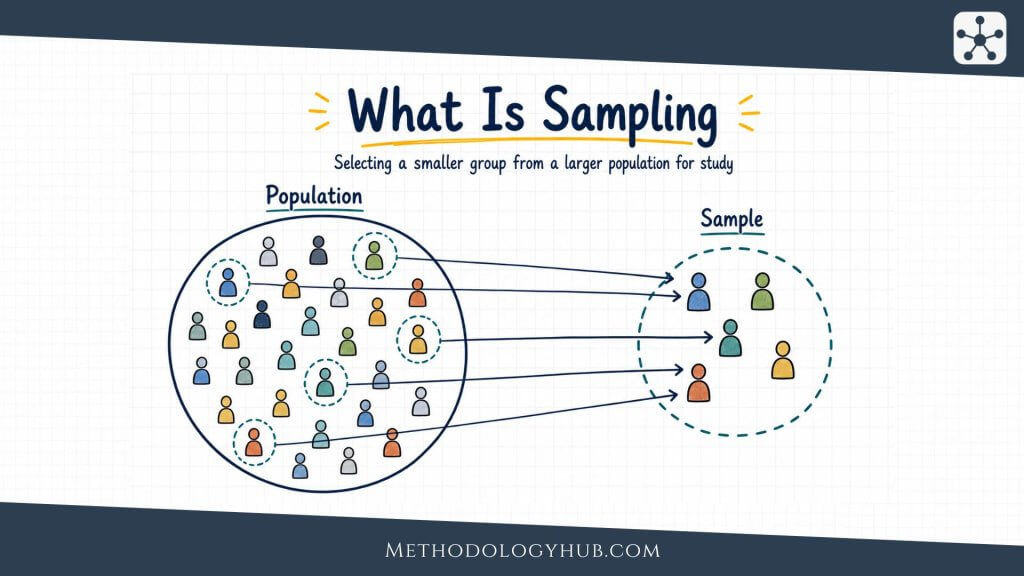
Four terms appear again and again in inferential statistics: Population, sample, parameter, and statistic. These terms are easiest to understand as a chain. A study usually begins with a population, which is the full group the researcher wants to say something about. Since that group is often too large to observe directly, the researcher works with a sample, meaning the smaller set of people, cases, records, or observations actually included in the study.

Inferential statistics then connects those two levels. A parameter describes the population, but it is usually unknown. A statistic is calculated from the sample and used to estimate that unknown value. For example, the average study time of all first-year students at a university would be a parameter. The average study time calculated from 200 surveyed students would be a statistic.

If a study measures reading scores in 300 students, the mean score of those 300 students is a statistic. The mean score of all students in the defined population is a parameter. The parameter is usually unknown. The statistic is available because it is calculated from observed data.

This vocabulary keeps claims in proportion. It reminds the reader that the data were observed in a particular sample, while the conclusion may be about a broader group. That shift is useful, but it has to be handled carefully.

Descriptive vs Inferential Statistics

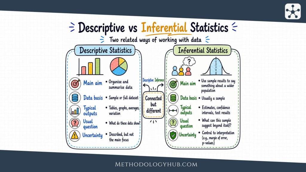
Descriptive and inferential statistics are closely connected, but they do different jobs. Descriptive statistics summarise the data that have been collected. Inferential statistics use those data to make conclusions about something beyond the observed sample.

A researcher usually begins with description. Before testing a hypothesis or estimating a population value, they need to understand the dataset. What is the average score. How spread out are the scores. Are there missing values. Are the groups similar in size. Descriptive statistics answer these first questions.

What descriptive statistics do

Descriptive statistics organise and summarise observed data. They include measures such as the mean, median, mode, range, variance, standard deviation, and percentages. They also include tables, charts, and graphs that show patterns in the data.

If a researcher reports that 120 students in a sample had an average exam score of 74, that statement is descriptive. It tells the reader what happened in the sample. It does not yet say whether all students in the population would have a similar average.

What inferential statistics do

Inferential statistics take the next step. They ask what the sample result suggests about the population. The researcher may estimate the population mean, calculate a confidence interval, test whether two groups differ, or examine whether two variables are associated beyond the observed dataset.

Suppose the same sample of 120 students is used to estimate the average exam score of all students taking the course. The researcher might calculate a confidence interval from 71 to 77. That interval does not describe only the 120 students. It gives a range of plausible values for the population mean, based on the sample and the assumptions of the method.

Aspect	Descriptive statistics	Inferential statistics
Main task	Summarise observed data	Draw conclusions beyond observed data
Focus	The available dataset	The wider population or process
Typical tools	Mean, median, standard deviation, charts	Confidence intervals, p-values, tests, models
Uncertainty	Usually described informally	Handled through probability and sampling theory

Example comparing both approaches

Imagine a psychology study measuring anxiety scores before and after a short intervention. The descriptive part may report the average before score, average after score, and the average change for the participants who completed the study. Those numbers describe what was observed.

The inferential part asks a broader question. Is the observed decrease large enough, relative to sample size and variation, to suggest that the intervention is associated with a real decrease in the population from which the participants were drawn. A paired-samples t-test or a confidence interval for the mean change could help answer that question.

The two approaches work together. Description gives the reader a clear view of the data. Inference gives a structured way to interpret what the data may suggest beyond the sample.

Core Concepts in Inferential Statistics

Inferential statistics becomes easier once a few core concepts are clear. These concepts explain why sample results differ, why uncertainty appears even in careful studies, and why statistical methods rely on assumptions. Without this foundation, tests and formulas can feel like separate procedures. With it, they begin to look like parts of the same logic.

Sampling error

Sampling error is the difference between a sample statistic and the true population parameter that occurs because a sample was used. It is not the same as a mistake. Even a well-selected random sample can differ from the population by chance.

Imagine drawing one sample of 100 students and calculating the average number of hours they study per week. If a second researcher draws another sample of 100 students from the same population, the average will probably be slightly different. Both samples may be valid. They are simply different samples.

Sampling distributions

A sampling distribution is the distribution of a statistic across many possible samples. The idea can sound abstract at first, but it is the basis for many inferential methods. If researchers could repeatedly draw samples of the same size from the same population, each sample would produce its own mean, proportion, correlation, or regression coefficient. Those values would form a distribution.

Inferential statistics uses that imagined distribution to judge how much sample results tend to vary. Standard errors, confidence intervals, and many hypothesis tests depend on this idea.

Standard error

The standard error describes how much a statistic would vary from sample to sample. A smaller standard error means the estimate is usually more precise. A larger standard error means repeated samples would be expected to produce more spread in the estimate.

For a sample mean, the standard error is often written as:

This formula shows why larger samples usually produce more precise estimates. When n increases, the denominator becomes larger, and the standard error becomes smaller. That does not repair a biased sample, but it does reduce random sample-to-sample variation when the design is suitable.

Assumptions

Inferential methods depend on assumptions. These assumptions are not decorative details. They are the conditions under which the method gives a useful answer. A t-test, chi-square test, ANOVA, correlation tests, or regression tests all rely on assumptions about the data, the design, or the relationship being analysed.

Common assumptions include independence of observations, suitable measurement level, an appropriate sample size, and a reasonable match between the method and the shape of the data. Some methods also assume approximate normality or equal variances across groups.

The assumptions do not have to make a study perfect. They help the researcher judge whether a method fits the data well enough. If the fit is poor, the result may still be calculated, but it may not be meaningful.

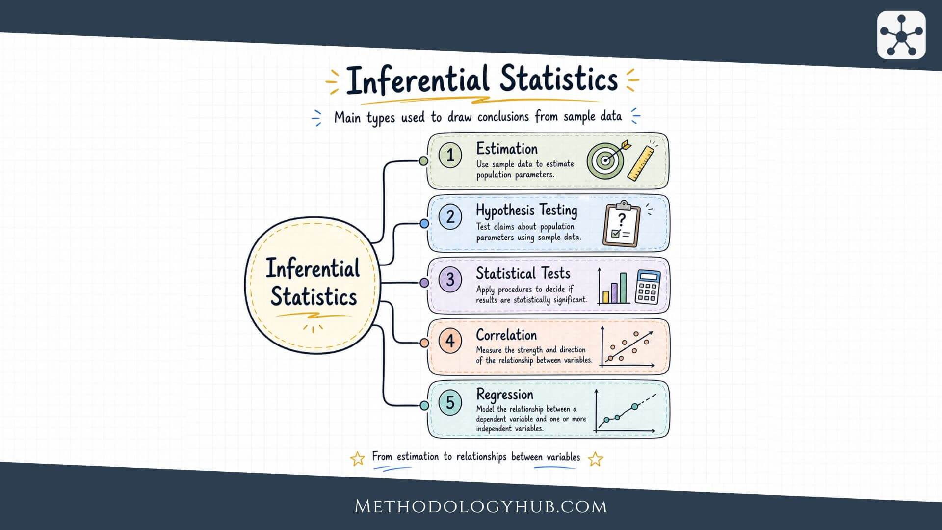
Types of Inferential Statistics

The main types of inferential statistics can be grouped into estimation, hypothesis testing, statistical tests, and model-based methods such as correlation and regression. These categories overlap in practice. A regression model, for example, can estimate coefficients, test hypotheses, and produce confidence intervals at the same time.

Estimation

Estimation uses sample data to approximate an unknown population value. The simplest form is point estimation, where one sample value is used as the best available estimate. A sample mean can estimate a population mean. A sample proportion can estimate a population proportion. A sample correlation can estimate a population correlation.

Because point estimates are rarely exact, researchers often add interval estimates. A confidence interval gives a range of plausible values for the population parameter. It tells the reader more than a point estimate alone because it includes uncertainty directly.

Hypothesis testing

Hypothesis testing evaluates a claim about a population using sample data. The researcher begins with a null hypothesis and an alternative hypothesis. The null hypothesis usually represents no difference, no effect, or no association. The alternative hypothesis represents the pattern the researcher is testing for.

The test then asks whether the sample evidence is unusual enough under the null hypothesis to reject it at a chosen significance level. This does not mean that the alternative hypothesis is proven with certainty. It means that the observed result would be unlikely if the null hypothesis were treated as true.

In practice, hypothesis testing is used when researchers compare groups, test associations, or evaluate whether an observed pattern could reasonably occur under a no-effect or no-difference assumption. For example, a researcher may test whether two teaching methods lead to different mean exam scores, whether two categorical variables are associated, or whether a correlation in a sample is strong enough to support a population-level conclusion.

A hypothesis test usually ends with one of two decisions: reject the null hypothesis or fail to reject the null hypothesis. The second wording is important. A non-significant result does not prove that there is no effect. It only means that the available sample evidence was not strong enough to reject the null hypothesis under the chosen test conditions.

Statistical tests

Statistical tests are the procedures used to evaluate evidence in hypothesis testing. Once the hypotheses are stated and the data are collected, the researcher chooses a test that fits the research question, the type of data, and the structure of the sample.

The choice of test is not arbitrary. A study comparing one sample mean with a known value needs a different test from a study comparing two independent groups. A study using categorical counts needs a different test again. The purpose of the test is to turn the observed data into a test statistic and p-value that can be interpreted against the significance level.

Many introductory tests can be grouped into two broad categories: parametric tests and nonparametric or categorical tests. Parametric tests are usually used with numerical data and make assumptions about the distribution of the data. Nonparametric tests are often used when those assumptions are not suitable, while categorical tests are used when the data are counts or categories rather than measured numerical values.

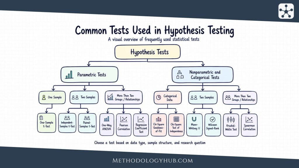
Parametric tests

Parametric tests are commonly used when the outcome variable is numerical and the data meet the main assumptions of the method. These tests often focus on means, relationships between numerical variables, or model coefficients.

• One-Sample t-Test: compares the mean of one sample with a known or hypothesised value.
• Independent-Samples t-Test: compares the means of two independent groups.
• Paired-Samples t-Test: compares two related measurements, such as before-and-after scores from the same participants.
• One-Way ANOVA: compares the means of three or more independent groups.
• Pearson Correlation: tests the strength and direction of a linear relationship between two numerical variables.
• Regression Coefficient Test: tests whether a predictor is statistically associated with an outcome in a regression model.

Nonparametric and categorical tests

Nonparametric and categorical tests are useful when the data are ordinal, strongly non-normal, based on ranks, or recorded as category counts. They are also used when the research question is about association between categories rather than comparison of means.

• Chi-Square Goodness-of-Fit Test: compares observed category counts with expected category counts.
• Chi-Square Test of Independence: tests whether two categorical variables are associated.
• Mann-Whitney U Test: compares two independent groups when a rank-based nonparametric approach is suitable.
• Wilcoxon Signed-Rank Test: compares two related measurements using ranks.
• Kruskal-Wallis Test: compares three or more independent groups using a rank-based approach.
• Spearman Correlation: tests a monotonic relationship between two variables using ranks.

The test name alone does not determine the quality of the analysis. A suitable test also depends on sample structure, measurement level, assumptions, and the way the result will be reported. For this reason, researchers usually begin with the research question, then identify the data type and group structure before selecting the statistical test.

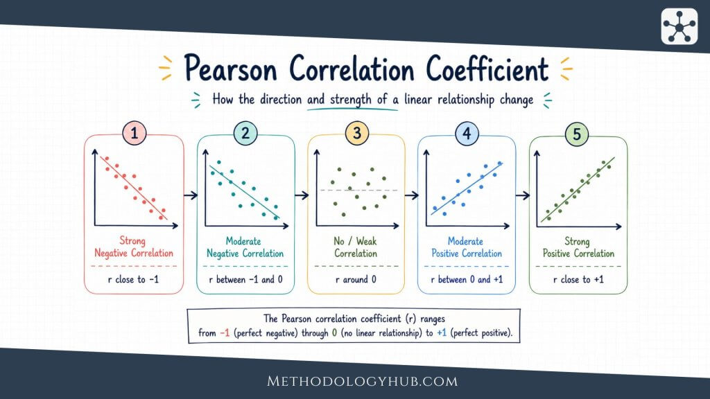
Correlation

Correlation is a statistical method used to measure the direction and strength of association between two variables. If two variables tend to increase together, the association is positive. If one variable tends to increase while the other decreases, the association is negative. If there is no clear pattern, the correlation is close to zero.

In most introductory contexts, correlation refers to Pearson’s correlation coefficient, usually written as r. It ranges from -1 to +1. A value near +1 shows a strong positive linear association, a value near -1 shows a strong negative linear association, and a value near 0 shows little or no linear association. Correlation describes association, not causation.

Regression

Regression is a statistical method used to model the relationship between an outcome variable and one or more predictor variables. It is often used when a researcher wants to estimate how much the outcome changes as a predictor changes. For example, a study might use regression to model exam score from study time.

In simple linear regression, there is one predictor and one outcome. In multiple regression, there are two or more predictors. Regression produces coefficients that describe the estimated relationship between the variables, such as the slope of a line. These coefficients can then be interpreted in relation to the research question, the research data, and the assumptions of the model.

Estimation

Estimation is often the most intuitive part of inferential statistics because it begins with a simple question: what is the population value likely to be. A researcher may want to estimate an average, a proportion, a difference between two means, a correlation, or a regression coefficient. In each case, the sample provides the available evidence.

Point estimation

A point estimate is a single value used to estimate a population parameter. If a sample of 80 plants has a mean height of 22.4 cm, then 22.4 cm is a point estimate of the population mean height. If 38 out of 100 survey participants report using a library database weekly, then 0.38 is a point estimate of the population proportion.

Point estimates are useful because they give a clear numerical result. They are also incomplete on their own. A point estimate does not show how much uncertainty surrounds it. A sample mean of 22.4 cm based on 30 plants does not carry the same precision as the same mean based on 3,000 plants.

Interval estimation

Interval estimation adds a range around the estimate. Instead of giving only one value, it gives a lower and upper bound. The most common interval estimate is the confidence interval.

A confidence interval for a mean might be written as 21.7 cm to 23.1 cm. This does not mean every plant in the population falls inside that range. It means the range is used to estimate the population mean, based on the sample result, sample size, variation, and selected confidence level.

Confidence intervals

A confidence interval is built from a point estimate, a standard error, and a critical value. A common structure is:

The confidence level is often 95%, although other levels can be used. In repeated sampling, a method that produces 95% confidence intervals would capture the true population parameter in about 95% of those intervals, assuming the method’s conditions are met.

For beginners, the safest way to read a confidence interval is to focus on plausible values. A narrow interval suggests a more precise estimate. A wide interval suggests more uncertainty. The location of the interval also helps interpretation. If a confidence interval for a mean difference lies entirely above zero, it suggests a positive difference under the method used. If it crosses zero, the evidence for a non-zero difference is weaker in that analysis.

Margin of error

The margin of error is the distance between the point estimate and the edge of the confidence interval. If a sample proportion is 0.52 and the confidence interval is 0.48 to 0.56, the margin of error is 0.04.

Margins of error are common in survey reporting, but the idea applies more broadly. They remind the reader that a sample estimate should not be treated as exact.

Standard error, margin of error, and confidence intervals together

The standard error describes the uncertainty of the estimate. The critical value adjusts that uncertainty for the confidence level. The margin of error is the amount added and subtracted from the estimate. The confidence interval is the final range.

Once these parts are separated, confidence intervals become less mysterious. They are not separate from estimation. They are estimation with uncertainty included.

Hypothesis Testing

Hypothesis testing is the part of inferential statistics that evaluates claims using sample evidence. It is often used when researchers want to compare groups, test whether an effect is present, or examine whether two variables are associated.

The language can feel formal at first, but the structure is quite simple. The researcher begins with a default position, collects or analyses data, and asks whether the sample result is unusual under that default position.

Null hypothesis

The null hypothesis is the starting claim in a hypothesis test. It often states that there is no difference, no effect, or no association in the population. For a comparison of two teaching methods, the null hypothesis may state that the population mean exam score is the same under both methods.

The null hypothesis is not always something the researcher believes. It is a reference point for the test. The sample result is judged against it.

Alternative hypothesis

The alternative hypothesis states what the researcher may conclude if the sample evidence is strong enough against the null hypothesis. It may state that there is a difference, an effect, or an association. Alternatives can be two-sided or one-sided.

A two-sided alternative says the population value differs from the null value in either direction. A one-sided alternative specifies a direction, such as greater than or less than. One-sided tests should be chosen before analysis, not after seeing which direction the sample result takes.

Test statistic and p-value

A test statistic summarises how far the sample result is from what the null hypothesis would predict, usually in standard error units. The exact test statistic depends on the method. A t-test produces a t statistic. ANOVA produces an F statistic. A chi-square test produces a chi-square statistic.

The p-value is the probability of observing a result at least as extreme as the sample result, assuming the null hypothesis is true and the model assumptions are satisfied. A small p-value means the observed result would be unusual under the null hypothesis. It does not give the probability that the null hypothesis is true.

Significance level alpha

The significance level, usually called alpha, is the threshold used for the statistical decision. A common value is 0.05. If the p-value is less than or equal to alpha, the result is often called statistically significant, and the null hypothesis is rejected.

Alpha should be chosen before looking at the results. Changing it after seeing the p-value makes the decision less trustworthy because the rule has been adjusted to the outcome.

Type I error, Type II error, and statistical power

A Type I error occurs when a true null hypothesis is rejected. If alpha is 0.05, the method is set up to allow a 5% Type I error rate under the null hypothesis across repeated tests of the same kind.

A Type II error occurs when a false null hypothesis is not rejected. This can happen when the sample is too small, the effect is weak, the data are noisy, or the method is not well matched to the design.

Statistical power is the probability of rejecting a false null hypothesis. Power tends to increase when the sample size is larger, the effect is stronger, the data are less variable, or the significance level is less strict. Power analysis is often used when planning a study because it helps researchers think about whether the design can detect an effect of a chosen size.

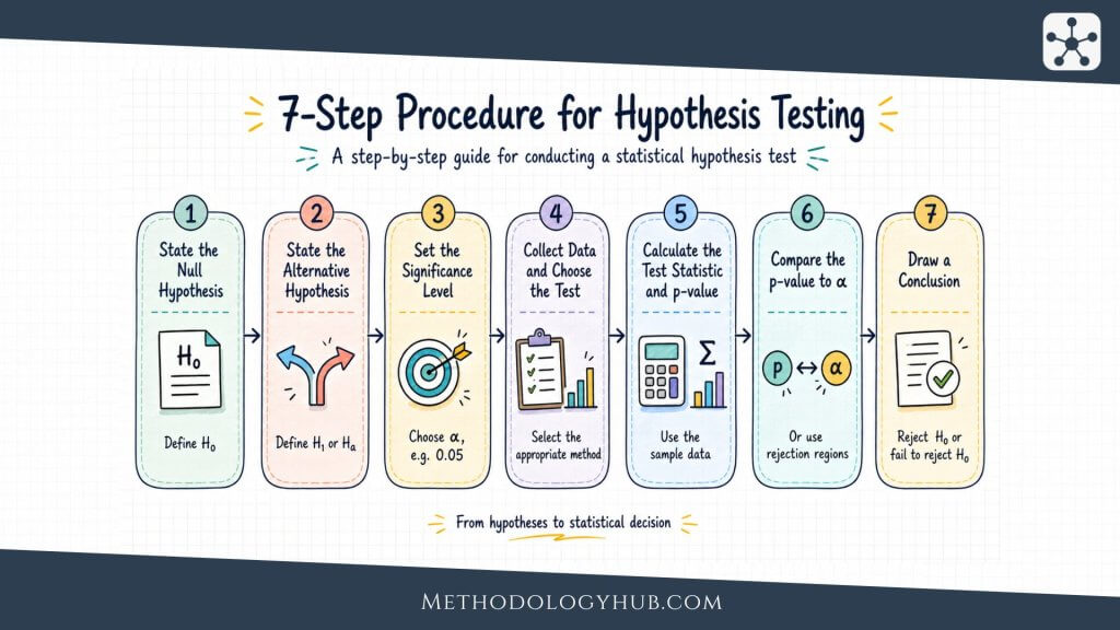
Steps in a hypothesis test

A basic hypothesis test usually follows a clear sequence:

• state the null and alternative hypotheses
• choose the significance level
• select a method that fits the data and question
• calculate the test statistic
• find the p-value or compare with a rejection rule
• make the statistical decision
• interpret the result in the study context

The last step is where many results need the most care. A test can reject or fail to reject a null hypothesis, but the researcher still has to interpret the size, direction, design, and uncertainty of the result. Statistical significance alone is not a complete interpretation.

Statistical Tests

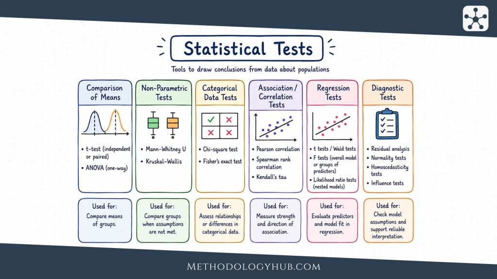
Statistical tests are formal procedures for comparing observed data with what would be expected under a statistical model. They are not interchangeable. The right test depends on the research question, variable type, sample structure, and assumptions.

T-test

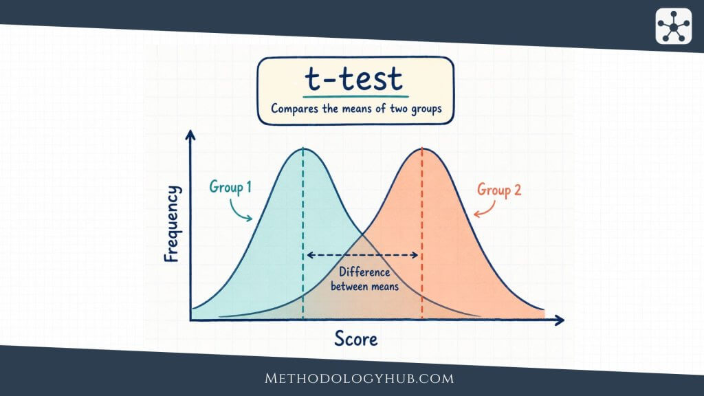
A t-test is used when the research question involves means and the data are quantitative. There are several forms. A one-sample t-test compares a sample mean with a hypothesised population mean. An independent-samples t-test compares means from two separate groups. A paired-samples t-test compares two related measurements, such as before and after scores from the same participants.

For example, an education researcher may compare exam scores between two independent groups of students taught with different lesson formats. If the outcome is a numerical score and the assumptions are suitable, an independent-samples t-test may be appropriate.

Chi-square test

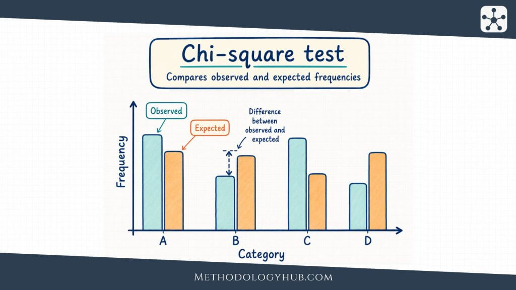
A chi-square test is used with categorical data. The chi-square goodness-of-fit test compares observed frequencies with expected frequencies in one categorical variable. The chi-square test of independence examines whether two categorical variables are associated.

For example, a biology study may compare observed genetic trait counts with expected Mendelian ratios. A sociology study may examine whether field of study is associated with preferred study location. In both cases, the data are counts in categories, not means.

ANOVA

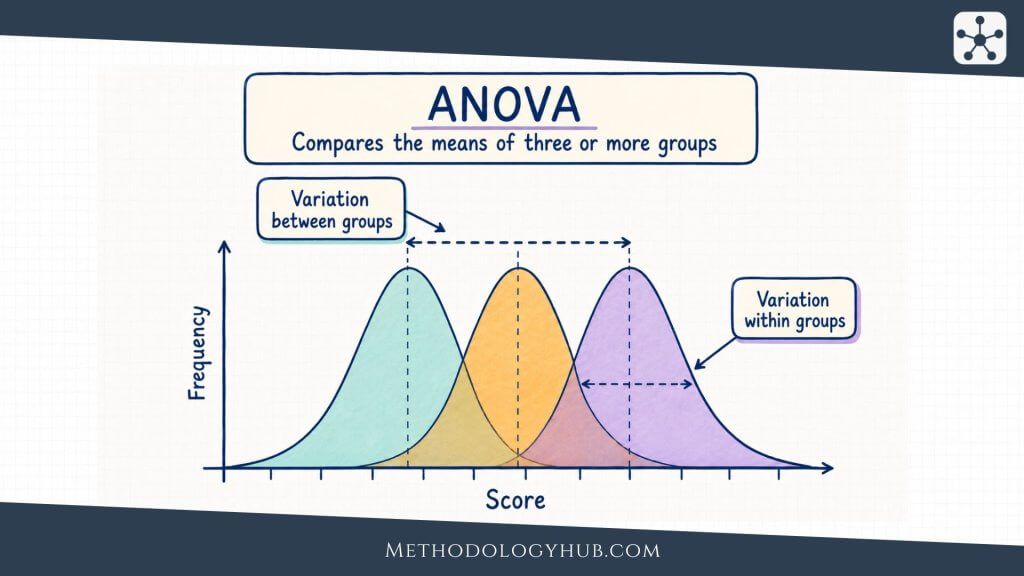
ANOVA stands for analysis of variance. It is commonly used to compare means across three or more groups. A one-way ANOVA tests whether at least one group mean differs from the others. It does this by comparing variation between groups with variation within groups.

The test statistic in ANOVA is the F statistic. If the ANOVA result is statistically significant, follow-up comparisons may be used to examine which groups differ. Those follow-up comparisons should be planned and interpreted carefully because multiple comparisons can increase the chance of false positives.

This overview gives only the first decision point. Researchers also need to consider sample size, independence, distributional shape, equal variances, expected cell counts, and the design of the study. The test should fit both the data and the claim.

Correlation

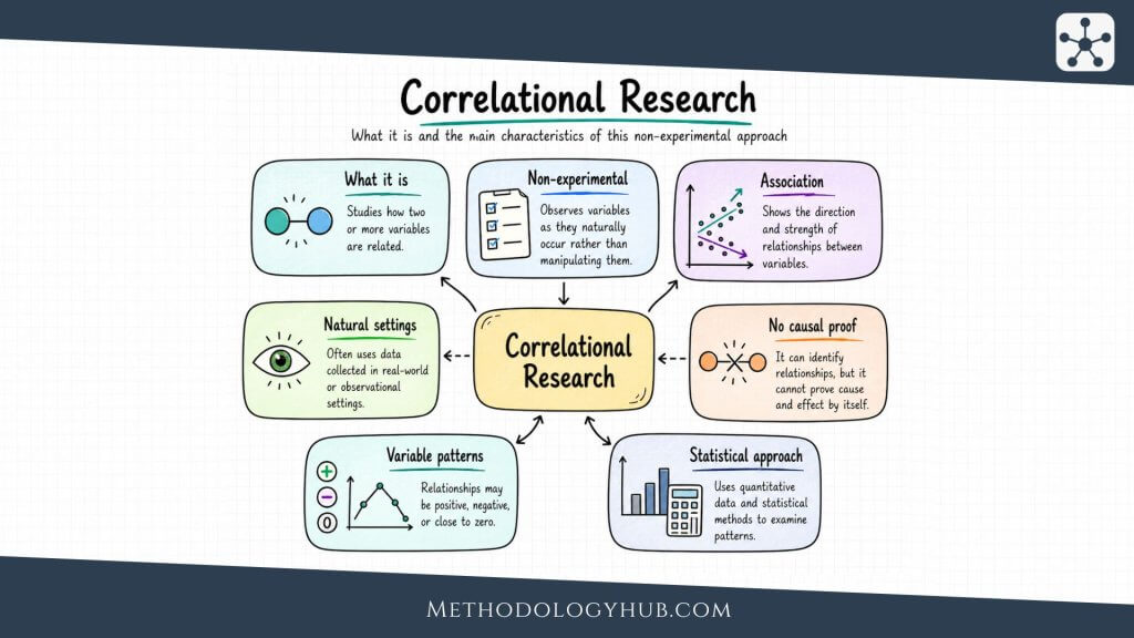
Correlation is a statistical method used to measure the direction and strength of association between two variables. It is used when a researcher wants to know whether values of one variable tend to move together with values of another variable.

For example, a researcher may examine the relationship between hours spent studying and exam score in a sample of students. If students who study more hours also tend to have higher scores, the correlation is positive. If one variable tends to increase while the other decreases, the correlation is negative. If there is no clear linear pattern, the correlation is close to zero.

Pearson correlation coefficient

In many introductory statistics contexts, correlation refers to Pearson’s correlation coefficient, usually written as r. Pearson’s r is used for linear association between two quantitative variables. Its values range from -1 to +1.

A value near +1 suggests a strong positive linear association. A value near -1 suggests a strong negative linear association. A value near 0 suggests little or no linear association. Correlation describes association, not causation, so it does not prove that one variable caused the other to change.

Correlation as descriptive and inferential

A sample correlation can be descriptive when it only summarises the observed dataset. In that case, it tells the reader how two variables were associated in the sample that was actually measured.

Correlation becomes inferential when the researcher uses the sample correlation to estimate a population correlation, calculate a confidence interval, or test a hypothesis about the population relationship. A common hypothesis test for correlation is:

• H0: rho = 0
• H1: rho is not equal to 0

Here, rho refers to the population correlation. The sample correlation r is used as evidence about rho.

Regression

Regression is a statistical method used to model the relationship between an outcome variable and one or more predictor variables. It is often used when a researcher wants to estimate how much an outcome changes when a predictor changes.

For example, a researcher may model exam score from study time. In that case, exam score is the outcome variable, and study time is the predictor variable. The regression model estimates the relationship between the two variables and gives a numerical coefficient for that relationship.

Simple linear regression

Simple linear regression has one outcome variable and one predictor variable. It fits a straight line through the data so that the researcher can describe the estimated relationship between the predictor and the outcome.

A simple linear regression model is often written as:

In this model, Y is the outcome, X is the predictor, beta0 is the intercept, beta1 is the slope, and the error term represents variation not explained by the line. The slope tells us the estimated change in Y for a one-unit increase in X.

Multiple regression

Multiple regression uses two or more predictor variables to model one outcome variable. It is useful when a researcher wants to examine a relationship while including several predictors in the same model.

For example, a study might model exam score using study time, prior achievement, attendance, and reading time. Each predictor receives its own coefficient. The coefficient estimates the relationship between that predictor and the outcome while the other predictors in the model are included.

Regression coefficients and inference

Regression coefficients describe estimated relationships between predictors and the outcome. In simple linear regression, the slope coefficient shows the estimated change in the outcome for each one-unit increase in the predictor.

Regression becomes inferential when researchers test coefficients or calculate confidence intervals around them. A common null hypothesis for a slope is:

• H0: beta1 = 0
• H1: beta1 is not equal to 0

If the slope is statistically different from zero, the researcher has evidence of a linear relationship between the predictor and outcome in the population, under the model assumptions. A confidence interval for the slope shows a range of plausible population slopes.

Model fit and residuals

Regression also asks how well the model fits the data. One familiar measure is R squared, which describes the proportion of variation in the outcome associated with the predictors in the model.

Residuals are the differences between observed values and values predicted by the model. They are useful because they reveal where the model fits poorly. They can also show patterns that suggest the relationship is not linear, the variability changes across values of the predictor, or an unusual observation is influencing the model.

Examples of Inferential Statistics

Examples of inferential statistics show how the same logic appears across different fields. The details change, but the basic movement stays the same: a researcher studies a sample, calculates a statistic, and then makes a careful statement about a wider population or process.

Example from medicine

A clinical study may measure blood pressure before and after a treatment in a sample of patients. Descriptive statistics show the average change in the sample. Inferential statistics can estimate the mean change in the wider patient population and test whether the change differs from zero.

A confidence interval is especially useful here because it shows the range of plausible treatment effects. A p-value can support a statistical decision, but the interval gives more detail about the size and precision of the estimated change.

Example from education

An education researcher may compare exam scores between students who used two different study approaches. If the groups are independent and the outcome is numerical, an independent-samples t-test may be used. The test examines whether the observed difference between sample means is larger than expected under a null hypothesis of no population difference.

Example from psychology

A psychology study may measure anxiety scores before and after a guided intervention. Because the same participants are measured twice, the observations are related. A paired-samples t-test can examine whether the mean change differs from zero in the population represented by the sample.

Example from biology

A genetics exercise may compare observed trait counts with expected ratios. A chi-square goodness-of-fit test can evaluate whether the observed counts differ from the expected counts more than would usually be expected by chance under the model.

Example from sociology

A sociology researcher may compare mean belonging scores across students from several types of institutions. Because there are more than two groups, ANOVA may be appropriate. If the ANOVA result is statistically significant, follow-up comparisons can examine where the differences appear.

How to Interpret Inferential Statistics

Interpreting inferential statistics means reading the result in relation to the research design, rather than only the formula. A p-value, confidence interval, or model coefficient is never floating alone. It belongs to a sample, a measurement process, a set of assumptions, and a research question.

Statistical significance

Statistical significance means that a result met the chosen decision rule for a hypothesis test. If alpha is 0.05 and the p-value is 0.03, the result is statistically significant by that rule. This does not automatically mean the effect is large, useful, or theoretically convincing.

A tiny effect can become statistically significant in a very large sample. A meaningful effect can fail to reach statistical significance in a small or noisy sample. For that reason, statistical significance should be read together with effect size, confidence intervals, study design, and prior knowledge.

Effect size

Effect size describes the magnitude of a result. It asks how large the difference, association, or change is. Different methods use different effect sizes. Mean differences, standardised mean differences, odds ratios, correlation coefficients, and regression slopes can all communicate magnitude in different contexts.

Effect size helps prevent a result from being interpreted only as significant or non-significant. It gives the reader a clearer sense of scale.

Practical interpretation

Practical interpretation connects the statistical result back to the study setting. A confidence interval may show that an estimated difference is small. A regression slope may be statistically significant but too uncertain to support a strong conclusion. A correlation may be clear but still limited to association.

Good interpretation uses careful language. It avoids turning one result into more than the design can support. It also avoids hiding useful evidence just because a single threshold was not crossed.

Conclusion

Inferential statistics gives researchers a way to use sample data without pretending that the sample is the whole population. It begins with a simple problem: research usually observes only part of the group it wants to understand. From there, inferential methods help estimate population values, test claims, compare groups, and examine relationships between variables.

The central ideas are connected. A sample statistic estimates a population parameter. Sampling error creates uncertainty. Standard errors help describe that uncertainty. Confidence intervals turn estimates into ranges. Hypothesis tests evaluate claims. Statistical tests, correlation, and regression apply those ideas to different research questions.

The strongest use of inferential statistics is careful rather than mechanical. A result should be read with the sample, assumptions, effect size, interval width, and study design in view. When those pieces are kept together, inferential statistics becomes less like a set of formulas and more like a disciplined way of reasoning from evidence.

Sources and Recommended Readings

If you want to go deeper into inferential statistics, the following scientific publications provide useful discussions of estimation, hypothesis testing, confidence intervals, statistical tests, and the interpretation of statistical evidence.

• An Introduction to Inferential Statistics – A review article introducing p-values, confidence intervals, and common statistical tests.
• Inferential Statistics – A clinical research article explaining inferential methods for readers new to research statistics.
• Understanding Inferential Statistics – A book focused on the logic of statistical inference, hypothesis testing, common tests, and correlation or regression.
• Inferential Statistics – A Springer chapter on parameters, sample statistics, estimation, and inference.
• Inferential Statistics Is an Unfit Tool for Interpreting Data – A critical article on the limits of null hypothesis significance testing and statistical benchmarks.
• For a proper use of frequentist inferential statistics in public health and epidemiology research – A framework for interpreting frequentist inference in health research.
• Hypothesis-Testing Demands Trustworthy Data – A Simulation Approach to Inferential Statistics Advocating the Research Program Strategy – A psychology article on hypothesis testing, inference, and research programs.
• A critique of the usefulness of inferential statistics in applied behavior analysis – A scientific critique of how inferential statistics are used in applied behavior analysis.
• Medical Statistics Series: Inferential Statistics (Part-I) – A medical statistics article covering hypotheses, errors, confidence intervals, p-values, and normality.
• Against Inferential Statistics: How and why current statistics teaching gets it wrong – A research output discussing arguments against current approaches to teaching inferential statistics.