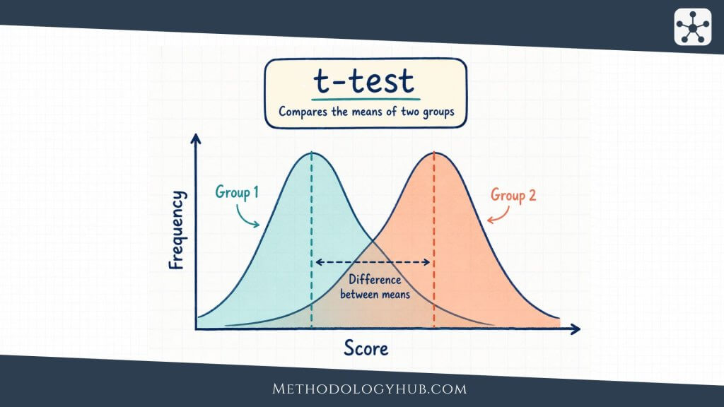
t-Test is a statistical test used to compare means when a research question is about one sample, two independent groups, or two related measurements. It is one of the most familiar procedures in inferential statistics because many studies ask whether an average score, time, measurement, or scale value differs from another average or from a stated benchmark.
This article explains what a t-Test is, how the main types of t-tests differ, which assumptions need attention, when to use a t-Test, how the formula works, how to calculate a simple example, and how to interpret and report the result in academic writing.
What Is a t-Test?
A t-Test is a statistical procedure for comparing a mean with another mean or with a hypothesised value. The test asks whether the observed difference is large enough, relative to variation in the data and the size of the sample, to count as evidence against a null hypothesis.
Imagine a teacher wants to know whether students in one class scored differently from the usual course average of 70. The class average is 74. At first, that looks higher. A t-Test asks a more careful question: could a sample average of 74 reasonably appear just because this class is one sample from a wider group of possible students, or is the difference large enough to suggest that the population mean is not 70?
t-Test definition
A t-Test is a hypothesis test for means that uses the t distribution. It is usually used when the outcome variable is numerical and the population standard deviation is unknown. The result is expressed through a t statistic, degrees of freedom, and a p-value.
The word mean is central here. A t-Test is not designed for category counts, rankings by themselves, or general relationships between two variables. If the question is about whether two categorical variables are associated, a chi-square test may be more suitable. If the question is about whether two numerical variables move together, a correlation test may fit better.
What the t statistic shows
The t statistic compares the observed mean difference with the amount of uncertainty around that difference. A difference of 4 points may look large in one study and small in another. If scores vary widely and the sample is small, a 4-point difference may be hard to interpret. If scores are consistent and the sample is larger, the same difference may provide stronger evidence.
This is why the t statistic is built from two parts: the difference being tested and the standard error of that difference. The standard error describes how much the sample mean or mean difference would be expected to vary from sample to sample. The t statistic puts the observed difference into that scale of uncertainty.
Why the t distribution is used
The t distribution is used because the population standard deviation is usually unknown in real research. Instead, the standard deviation is estimated from the sample. That extra uncertainty is especially noticeable in small samples, so the t distribution has heavier tails than the normal distribution. As sample size increases, the t distribution becomes closer to the normal distribution.
For beginners, the main idea is simple: the t-Test does not assume that the researcher knows the population spread exactly. It estimates spread from the sample, then accounts for the uncertainty that comes from doing so.
How a t-Test connects to statistical inference
A t-Test belongs to inferential statistics because it uses sample data to make a statement about a wider population or process. The sample mean is observed. The population mean is usually unknown. The test uses the sample result to judge whether a claim about the population mean is plausible under the null hypothesis.
This does not mean the test proves that the alternative hypothesis is true. It means the data are compared with a specific null model. The conclusion should therefore stay close to the study design, the sample, the assumptions, and the size of the observed difference.
Key Aspects of the t-Test
The t-Test becomes easier to understand when its main parts are seen as one process. A researcher starts with a question about a mean, writes hypotheses, checks the structure of the data, calculates a t statistic, and interprets the p-value in relation to a chosen significance level.
Each part has its own job. The hypotheses define the claim being tested. The standard error describes uncertainty. Degrees of freedom connect the result to the correct t distribution. The p-value gives a probability statement under the null hypothesis. The effect size and confidence interval help turn the test result into a more complete interpretation.
Mean difference
The mean difference is the comparison at the centre of the t-Test. In a one-sample t-Test, it is the sample mean minus the hypothesised population mean. In an independent-samples t-Test, it is the difference between two group means. In a paired-samples t-Test, it is the average of the differences within pairs.
The same number can mean different things depending on the research design. A difference between two unrelated groups is not the same as a change within the same participants. This is why the first step is not calculation. The first step is understanding what kind of comparison the data actually contain.
Null and alternative hypotheses
The null hypothesis usually states that there is no mean difference in the population, or that the population mean equals a stated value. The alternative hypothesis states the pattern that would receive support if the sample evidence is strong enough against the null hypothesis.
For a one-sample t-Test, the hypotheses may be H0: μ = 70 and Ha: μ ≠ 70. For two independent groups, the null hypothesis may state that the two population means are equal. For paired data, the null hypothesis may state that the mean difference between the two measurements is zero.
Standard error
The standard error describes the expected sample-to-sample variation of the mean or mean difference. A smaller standard error means the estimate is more precise. A larger standard error means the observed difference is surrounded by more uncertainty.
Standard error depends strongly on sample size and variability. Larger samples usually reduce the standard error. More variable data increase it. That is why a t-Test does not look only at whether two means are different. It asks whether the difference is large relative to the uncertainty in the estimate.
Formula: t = observed mean difference / standard error of the difference
Degrees of freedom
Degrees of freedom describe how much independent information is available for estimating variation. In a one-sample t-Test, the degrees of freedom are usually n – 1. If there are 25 observations, the test has 24 degrees of freedom.
Degrees of freedom affect the shape of the t distribution used for the p-value. With fewer degrees of freedom, the t distribution is wider because the sample gives less information about the population spread. With more degrees of freedom, the distribution becomes closer to the normal distribution.
p-value and significance level
The p-value is the probability of obtaining a result at least as extreme as the observed result, assuming the null hypothesis is true and the test assumptions are suitable. If the p-value is small, the observed result would be unusual under the null hypothesis.
The significance level, often written as α, is the decision threshold chosen before the test. A common value is 0.05. If p < 0.05, many researchers reject the null hypothesis. If p is larger, they fail to reject it. This wording is careful because a non-significant result does not prove that the null hypothesis is true.
Effect size and confidence interval
A t-Test can tell the reader whether the evidence is strong enough to reject a null hypothesis, but it does not by itself show how large or meaningful the difference is. For that, researchers often report an effect size and a confidence interval.
For two means, Cohen’s d is a common effect size. It expresses the mean difference in standard deviation units. A confidence interval gives a range of plausible values for the population mean difference. Together, these additions make the interpretation less dependent on the p-value alone.
Types of t-Tests
There are three main types of t-Tests in introductory statistics: the one-sample t-Test, the independent-samples t-Test, and the paired-samples t-Test. They all compare means, but they answer different research questions because the data are arranged differently.
The difference between them is not cosmetic. A one-sample test compares one sample with a benchmark. An independent-samples test compares two separate groups. A paired-samples test compares two linked measurements. Choosing the wrong one changes the meaning of the result.
One-sample t-Test
A one-sample t-Test compares the mean of one sample with a known or hypothesised value. The value may come from a previous study, a test norm, a policy benchmark, or a theoretical expectation.
For example, suppose a researcher studies whether a sample of 40 students has a mean reading score different from a national benchmark of 75. The sample mean is compared with 75, and the standard error is calculated from the sample standard deviation and sample size.
Independent-samples t-Test
An independent-samples t-Test compares the means of two groups that are not naturally linked. The observations in one group should not determine or match the observations in the other group. Two different classes, two treatment groups, or two separate participant groups are common examples.
For example, a researcher may compare exam scores between students who used printed study materials and students who used digital study materials. If each student belongs to only one group, and the outcome is numerical, an independent-samples t-Test may be suitable when the assumptions fit.
Welch’s t-Test
Welch’s t-Test is a form of independent-samples t-Test that does not assume equal population variances. It is often used when two independent groups have different standard deviations, different sample sizes, or both. Many software packages report both the equal-variance version and Welch’s version.
The practical difference is that Welch’s t-Test adjusts the degrees of freedom. This makes it a safer choice in many two-group situations where the equal-variance assumption is doubtful. The conclusion is still about a difference between two group means, but the calculation handles unequal spread more carefully.
Paired-samples t-Test
A paired-samples t-Test compares two related measurements. The same participants may be measured before and after an intervention, or each observation in one condition may be matched with a related observation in another condition.
In a paired-samples t-Test, the analysis is based on the differences within pairs. If students take a pre-test and a post-test, the test does not treat the pre-test scores and post-test scores as two unrelated groups. It calculates each student’s change score and tests whether the mean change differs from zero.
Choosing between the three types
The choice usually follows from the research question. One group compared with a benchmark suggests a one-sample t-Test. Two separate groups suggest an independent-samples t-Test. Two linked measurements suggest a paired-samples t-Test.
| Research situation | Typical t-Test | Example question |
|---|---|---|
| One sample mean compared with a stated value | One-sample t-Test | Is the average score different from 70? |
| Two separate group means | Independent-samples t-Test | Do two classes differ in average score? |
| Two related measurements | Paired-samples t-Test | Did scores change from pre-test to post-test? |
Assumptions of the t-Test
The assumptions of the t-Test describe the conditions under which the result can be interpreted with confidence. They do not demand perfect data. They ask whether the test is a reasonable match for the research question, the measurement scale, the sample structure, and the distribution of the outcome.
Assumptions should be considered before the result is interpreted. A p-value can be calculated even when the method does not fit the data well. The more important question is whether the calculated result answers the research question in a defensible way.
Numerical outcome variable
A t-Test is intended for a numerical outcome variable. The outcome should be measured on a scale where means and differences between values are meaningful. Test scores, response times, blood pressure, height, scale totals, and measured distances are common examples.
If the outcome is categorical, such as pass or fail, yes or no, or preferred option, a t-Test is usually not the right method. For categorical counts, a chi-square test or another categorical data method is often more suitable. If the outcome is ordinal with only a few ordered categories, a rank-based method may fit better.
Independence of observations
Independence means that one observation should not determine another observation unless the test is designed for paired data. In a one-sample t-Test and an independent-samples t-Test, each case should contribute one independent observation. If several scores come from the same student, class, family, clinic, or laboratory batch, ordinary t-Test calculations may treat related observations as if they were separate.
For a paired-samples t-Test, independence applies to the pairs rather than to the two values inside a pair. Each pair can contain related measurements, but the pairs themselves should usually be independent of one another.
Approximate normality
The t-Test assumes approximate normality in the relevant distribution. For a one-sample t-Test, the sample values should be reasonably normal, especially when the sample is small. For a paired-samples t-Test, the differences between paired measurements should be reasonably normal. For an independent-samples t-Test, the outcome should be reasonably normal within each group, especially in small samples.
This does not mean every dataset must look perfectly bell-shaped. The t-Test is often fairly tolerant of mild departures from normality, particularly when sample sizes are moderate or large and there are no extreme outliers. With very small samples, strong skew, or unusual points, the assumption deserves closer attention.
Similar variances for the equal-variance independent-samples t-Test
The classic independent-samples t-Test assumes that the two population variances are equal. In practice, this assumption is often checked by comparing group standard deviations, looking at plots, or using software output. If the groups have noticeably different spread, Welch’s t-Test is usually the safer option.
This assumption does not apply in the same way to the one-sample or paired-samples versions. It is mainly a concern when two independent group means are compared with the pooled-variance version of the test.
No extreme outliers
Because the t-Test works with means and standard deviations, unusual observations can influence the result. A single extreme value can pull the mean, increase the standard deviation, and change the t statistic.
Outliers should not be removed automatically. They should be checked against the data collection process, measurement instrument, and coding decisions. Sometimes an outlier is a data entry error. Sometimes it is a real observation. The decision to keep, correct, remove, or analyse it separately should be explained.
Suitable sampling and study design
A t-Test only speaks as well as the study design allows. A large p-value from a poorly sampled group does not prove that no difference exists. A small p-value from a biased sample does not repair the sampling problem. The sampling method, measurement quality, and research design shape the interpretation before the test is even calculated.
This is especially relevant for convenience samples, clustered observations, or studies with missing data. A t-Test can still be part of the analysis, but the conclusion should reflect how the data were collected.
When to Use a t-Test
A t-Test is appropriate when the research question is about comparing means and the outcome variable is numerical. The exact version depends on whether the study has one sample, two independent groups, or two related measurements.
Many beginner errors happen before calculation. A researcher may choose a t-Test simply because it is familiar, even though the question is about categories, ranks, three or more groups, or a relationship between variables. Starting with the research question prevents that mismatch.
Use a t-Test for one mean compared with a benchmark
Use a one-sample t-Test when one sample mean is compared with a stated value. The benchmark should be meaningful before the data are analysed. It may come from a norm, a previous study, a theoretical value, or a planned criterion.
For example, a researcher may test whether the average score of a sample differs from a standard score of 100. The t-Test asks whether the sample mean is far enough from 100, relative to sample variation, to reject the null hypothesis that the population mean equals 100.
Use a t-Test for two independent group means
Use an independent-samples t-Test when two separate groups are compared on a numerical outcome. The groups should be independent, meaning that a participant or case appears in only one group and is not matched to a case in the other group.
For example, a researcher may compare average reaction time between two teaching formats, two treatment conditions, or two age groups. If there are more than two groups, ANOVA is usually considered instead of running many separate t-tests.
Use a t-Test for two related measurements
Use a paired-samples t-Test when the same cases are measured twice or when observations are naturally paired. Pre-test and post-test designs are the most familiar example, but matched pairs also appear in medical, educational, and laboratory studies.
The paired-samples t-Test focuses on change or difference within each pair. This can be more precise than comparing two unrelated groups because each case acts as its own reference point. That advantage depends on the pairing being real and meaningful.
Use another method when the question changes
If the research question is about three or more means, ANOVA is usually a better starting point. If the question is about categorical counts, a chi-square test may fit. If the question is about association between two numerical variables, Pearson correlation, Spearman’s rank correlation, or regression tests may be more suitable.
If the outcome is ordinal, strongly skewed, or not well represented by a mean, a nonparametric test may be considered. The Mann-Whitney U Test is often discussed for two independent groups, although it does not answer exactly the same question as a t-Test.
Formula for the t-Test
The formula for a t-Test changes slightly across the one-sample, independent-samples, Welch, and paired-samples versions. The general idea remains the same: compare an observed mean difference with the standard error of that difference.
This shared structure is useful because it keeps the formulas from looking like unrelated procedures. In every version, a larger difference increases the absolute t value, while more uncertainty lowers it.
General formula
General structure: t = difference being tested / standard error of that difference
The numerator is the observed difference from the null value. The denominator is the standard error. The test therefore asks whether the observed difference is large relative to the uncertainty expected from sampling variation.
One-sample t-Test formula
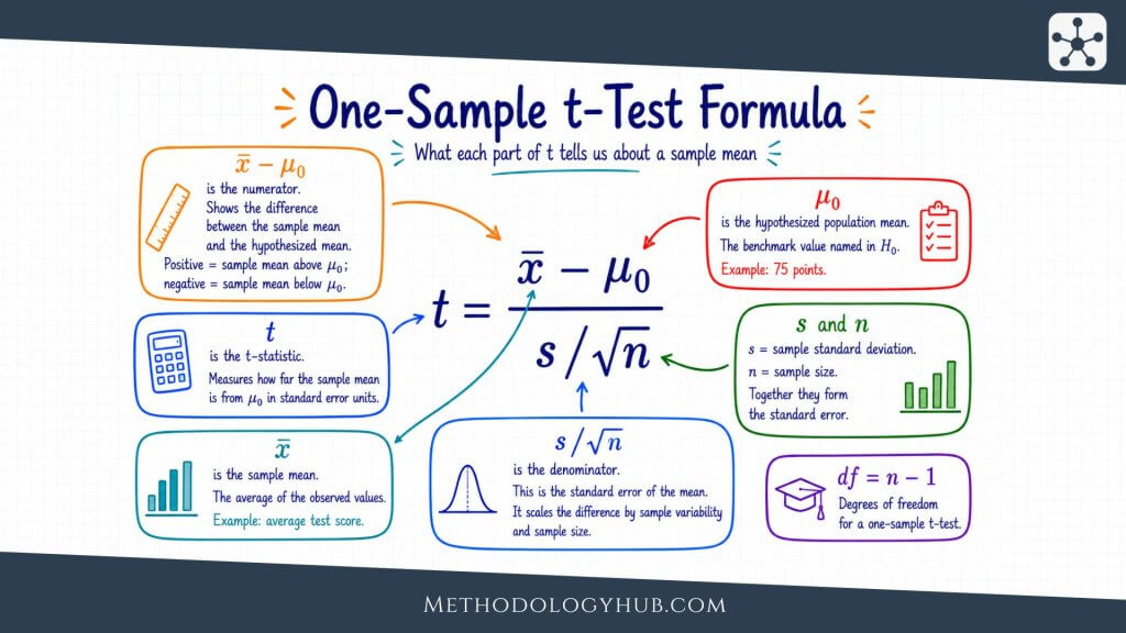
One-sample t-Test: t = (x̄ – μ0) / (s / sqrt(n))
In this formula, x̄ is the sample mean, μ0 is the hypothesised population mean, s is the sample standard deviation, and n is the sample size. The denominator, s / sqrt(n), is the standard error of the sample mean.
Paired-samples t-Test formula
Paired-samples t-Test: t = d̄ / (sd / sqrt(n))
Here, d̄ is the mean of the paired differences, sd is the standard deviation of those differences, and n is the number of pairs. This formula shows why the paired test is really a one-sample t-Test applied to difference scores.
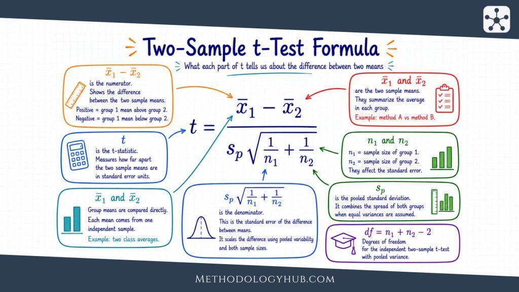
Independent-samples t-Test idea
For two independent groups, the numerator is the difference between the two group means. The denominator is the standard error of that difference. In the equal-variance version, the two group variances are pooled into one estimate. In Welch’s version, the standard error uses the two group variances separately.
The formulas differ because the assumptions differ. The equal-variance version assumes the groups share a common population variance. Welch’s version avoids that assumption and adjusts the degrees of freedom.
What the formula does in plain language
The formula is not trying to decide whether two numbers are exactly equal. Sample means are almost never exactly equal. Instead, the formula asks whether the observed difference is large compared with the noise expected from sampling variation.
If the difference is small and the data are variable, the t value will be close to zero. If the difference is large and the data are precise, the absolute t value will be larger. The p-value then tells the reader how unusual that t value would be under the null hypothesis.
Example Usage of the t-Test
A small example can show how the logic of a t-Test works. The numbers below are simple on purpose. In a real study, the researcher would also describe the sampling method, inspect the data, check assumptions, and report uncertainty around the estimate.
Suppose a teacher wants to know whether the average score in a class differs from a school benchmark of 70. Ten students take a short assessment. Their scores are shown below.
| Student | Score |
|---|---|
| A | 68 |
| B | 72 |
| C | 75 |
| D | 70 |
| E | 77 |
| F | 73 |
| G | 74 |
| H | 69 |
| I | 76 |
| J | 71 |
Step 1: State the hypotheses
The null hypothesis states that the population mean score is 70. The alternative hypothesis states that the population mean score is different from 70. Because the teacher is interested in either a higher or lower difference, this is a two-sided test.
Null hypothesis: H0: μ = 70
Alternative hypothesis: Ha: μ ≠ 70
Step 2: Calculate the sample mean and standard deviation
The ten scores have a sample mean of 72.5. Their sample standard deviation is approximately 3.03. The sample mean is therefore 2.5 points above the benchmark.
That 2.5-point difference is the numerator of the t statistic. To interpret it, the researcher also needs the standard error, which describes how much a sample mean would be expected to vary.
Step 3: Calculate the standard error
Standard error:
SE = s / sqrt(n)
SE = 3.03 / sqrt(10)
SE = 0.96
The standard error is about 0.96. This means the observed difference of 2.5 points is a little more than two and a half standard errors above the null value.
Step 4: Calculate the t statistic
t statistic:
t = (72.5 – 70) / 0.96
t = 2.61
The degrees of freedom for a one-sample t-Test are n – 1. With 10 students, df = 9. Statistical software would use t = 2.61 and df = 9 to calculate the p-value.
Step 5: Interpret the p-value
For this example, a two-sided one-sample t-Test gives a p-value of about .028. If the significance level was set at .05 before the analysis, the p-value is below the threshold. The researcher would reject the null hypothesis.
The statistical interpretation is not simply that the class average is 72.5. That part is descriptive. The t-Test result says that, under the test assumptions, the sample provides evidence that the population mean differs from 70.
Step 6: Add context to the result
The result should still be read cautiously. The sample is small, and the example does not describe how the students were selected. The difference is positive, but the conclusion should not claim that a teaching method caused the difference unless the study design supports that claim.
A short report could read: “A one-sample t-Test showed that the mean score in the sample was higher than the benchmark of 70, t(9) = 2.61, p = .028. The sample mean was 72.5, suggesting a positive difference of 2.5 points under the assumptions of the test.”
Interpretation of the t-Test
Interpreting a t-Test means more than checking whether p is below .05. The reader needs to know what was compared, which direction the difference took, how large the difference was, how uncertain it was, and whether the design supports the conclusion.
A good interpretation begins with the research question and returns to it at the end. If the study asked whether two teaching formats produced different mean scores, the interpretation should name those formats and the score. If the study asked whether a mean differs from a benchmark, the interpretation should name the benchmark and the observed mean.
Interpreting statistical significance
A statistically significant t-Test result means that the observed difference would be unusual under the null hypothesis, given the assumptions of the test. It does not mean the difference is automatically large, useful, causal, or practically important in the study setting.
A non-significant result means that the sample did not provide enough evidence to reject the null hypothesis. It does not prove that the means are exactly equal. Small samples, noisy measurements, and weak study designs can all make real differences hard to detect.
Interpreting direction
The sign of the mean difference tells the direction. In a one-sample t-Test, a positive difference means the sample mean is higher than the hypothesised value. A negative difference means it is lower. In a two-group t-Test, direction depends on which group mean is subtracted from which.
The report should make the direction clear in words. A sentence such as “Group A scored higher than Group B” is easier to read than a statement that only reports a positive t value. Direction is part of interpretation, not a detail to leave hidden in the formula.
Interpreting effect size
Effect size helps the reader judge how large the difference is. Cohen’s d is often used for t-Tests. It expresses the difference in standard deviation units. For paired-samples tests, the effect size should match the paired design rather than treating the two sets of observations as independent.
Labels such as small, medium, and large can be useful for teaching, but they should not replace context. A small mean difference may be meaningful in some fields if the outcome is difficult to change or the measurement is highly consequential. A large-looking difference may be less persuasive if the sample is biased or the confidence interval is wide.
Interpreting confidence intervals
A confidence interval gives a range of plausible values for the population mean difference. If a 95% confidence interval for a mean difference is 0.6 to 4.4, the estimate suggests a positive difference, but also shows that the exact size is uncertain.
Confidence intervals are especially useful because they keep direction, size, and uncertainty together. A p-value gives a decision against a null value. A confidence interval shows what values remain plausible under the method used.
Writing the result in academic style
A concise report usually includes the test type, means or mean difference, t statistic, degrees of freedom, p-value, and sometimes the confidence interval and effect size. The amount of detail depends on the level of the work and the role of the test in the study.
Example report: Students in the post-test condition had a higher mean score than in the pre-test condition, t(29) = 3.14, p = .004, 95% CI [1.20, 5.80]. The mean increase was 3.5 points.
This wording gives the reader the direction, test statistic, p-value, confidence interval, and plain-language meaning. It does not claim more than the design can support.
t-Test Compared with Other Statistical Tests
The t-Test sits inside a wider family of statistical tests. It is useful, but it is not a general solution for every comparison. The best test depends on the variable type, number of groups, independence structure, and research question.
Comparing the t-Test with nearby methods helps clarify its role. The boundaries are especially important for students because several tests may appear in the same software menu even though they answer different questions.
t-Test and ANOVA
A t-Test is usually used for one mean or two means. ANOVA is used when the researcher wants to compare means across three or more groups. Running several separate t-tests across many groups can increase the chance of false positives because each test adds another opportunity to reject a true null hypothesis.
ANOVA first asks whether there is evidence that at least one group mean differs. If the result is statistically significant, follow-up comparisons can then examine where the differences appear. Those follow-up comparisons should be planned and adjusted appropriately.
t-Test and Mann-Whitney U Test
The Mann-Whitney U Test is often considered when two independent groups are compared and the outcome is ordinal, strongly non-normal, or better analysed through ranks. It is not simply a t-Test without assumptions. It works with ranks and answers a different kind of question about the distributions of the two groups.
If the research question is specifically about means and the data are reasonably suited to a t-Test, a t-Test may still be appropriate. If the measurement scale or distribution makes means less informative, a rank-based method may give a better answer.
t-Test and correlation tests
A t-Test compares means. Correlation tests examine association between variables. A study asking whether average test scores differ between two groups is a mean comparison. A study asking whether study time is associated with test score is a correlation question.
Some correlation tests use a t statistic internally, but that does not make them t-Tests in the ordinary sense. The research question determines the method. For rank-based association, Kendall’s tau or Spearman’s correlation may be considered.
t-Test and regression tests
Regression can compare groups when a categorical predictor is included in a model, and it can also adjust for other variables. A two-group t-Test and a simple regression with one two-level predictor are closely related, but regression becomes more flexible when the research question includes several predictors, control variables, interactions, or prediction.
If the only question is whether two independent group means differ, a t-Test may be enough. If the question involves several variables at once, regression analysis may match the design more directly.
Conclusion
The t-Test gives researchers a structured way to compare means while keeping sample variation visible. It is used for one sample compared with a benchmark, two independent groups, or two related measurements. In each case, the test compares an observed mean difference with the standard error of that difference.
The strength of the t-Test is its clear link between a research question and a statistical decision. The researcher states the hypotheses, chooses the correct version of the test, checks whether the assumptions are reasonable, calculates the t statistic, and interprets the p-value together with the mean difference, confidence interval, and effect size.
Used well, a t-Test is not just a calculation. It is a way of asking whether a mean difference is large enough, relative to uncertainty, to support a population-level interpretation. The final conclusion should still stay close to the sample, the measurement process, and the design of the study.
FAQs on t-Test
What is a t-Test?
A t-Test is a statistical test used to compare means. It is commonly used when the outcome variable is numerical and the population standard deviation is unknown.
When should I use a t-Test?
Use a t-Test when the research question is about a mean or mean difference, the outcome is numerical, and the data structure fits a one-sample, independent-samples, or paired-samples comparison.
What are the three main types of t-Tests?
The three main types are the one-sample t-Test, independent-samples t-Test, and paired-samples t-Test. Welch’s t-Test is an important version of the independent-samples t-Test used when equal variances are doubtful.
What assumptions does a t-Test have?
A t-Test generally assumes a numerical outcome, independence of observations or pairs, approximate normality in the relevant distribution, and no extreme outliers. The equal-variance independent-samples t-Test also assumes similar variances across groups.