What Is Statistical Analysis: Methods, Types & Examples

Statistical analysis is the process of working with quantitative data so that observations can be organised, examined, and interpreted with care. In research, it usually begins long before a calculation is made. A researcher has to decide what is being studied, which variables can represent that question, how the data will be collected, and which method can answer the question without stretching the evidence too far.

This article explains what statistical analysis is, the key types of statistical analysis, how descriptive and inferential approaches work, how the analysis process is usually organised, which statistical methods are often used, and how statistical results are interpreted and reported in academic writing.

What Is Statistical Analysis?

Statistical analysis is a systematic way of examining numerical information. It includes preparing data, summarising what has been observed, choosing suitable statistical methods, and interpreting the results in relation to a research question. The same phrase can refer to a short descriptive summary or to a more complex model, but in academic work it usually describes the full movement from data to interpretation.

A researcher may begin with a question such as whether two teaching approaches are associated with different test scores, whether a treatment group shows a change over time, or whether rainfall and crop yield tend to vary together across several regions. Statistical analysis does not answer these questions by intuition alone. It turns the research question into measurable variables, examines the data structure, and applies methods that fit the design.

Statistical analysis definition

Statistical analysis means collecting, preparing, summarising, modelling, and interpreting quantitative data with statistical methods. It is used to describe datasets, estimate unknown values, test hypotheses, compare groups, examine relationships, and express uncertainty.

That definition is broad because statistical analysis is not one single calculation. A frequency table, a mean, a standard deviation, a confidence interval, a t-test, a chi-square test, a regression analysis, and a time series model can all belong to statistical analysis. What connects them is the attempt to read data in a structured way rather than treating isolated numbers as self-explanatory.

The word analysis also signals that the researcher has to make choices. A dataset does not announce its own method. A set of examination scores might be summarised with a mean and standard deviation, compared across two groups with a t-test, compared across several groups with ANOVA, or modelled with regression if several predictors are involved. The choice depends on the question, the variables, the sample, and the assumptions that can reasonably be made.

Data, variables, and observations

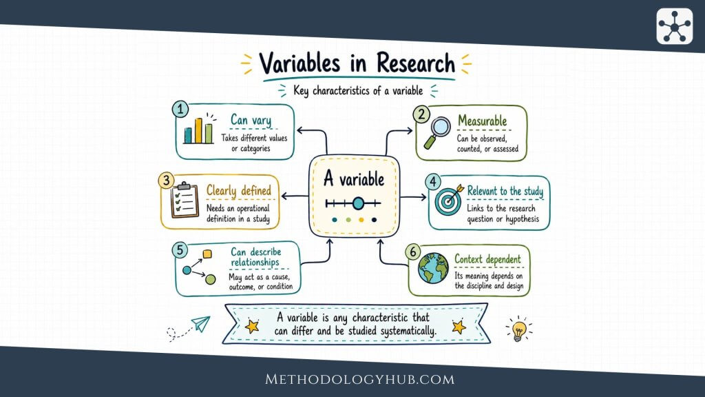
Statistical analysis begins with observations. An observation is one recorded case, such as one student, one patient, one plant, one school, one soil sample, or one measurement occasion. Each observation contains values for one or more variables. A variable is a characteristic that can differ across observations, such as age, score, height, temperature, diagnosis, response category, or time point.

These ideas are easier to follow in a small study. Suppose a researcher records reading scores, age, and study time for 120 students. Each student is an observation. Reading score, age, and study time are variables. The full table is the dataset. Statistical analysis then asks what can be learned from that table, while keeping the design and limits of the research data in view.

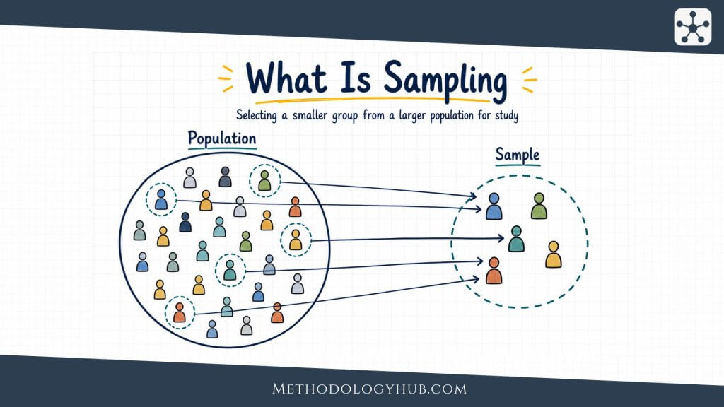
Sample and population

Many studies analyse a sample because the full population cannot be measured. The population is the complete group the researcher wants to understand. The sample is the smaller group actually observed. If a study records results from 300 students to learn about all students in a district, the 300 students form the sample, while all students in the district form the population.

This distinction shapes interpretation. A mean calculated from the sample describes the observed students. If the researcher uses that mean to estimate the district average, the claim has moved beyond description. At that point, statistical analysis has to handle uncertainty, because another sample might have produced a different value.

Types of Statistical Analysis

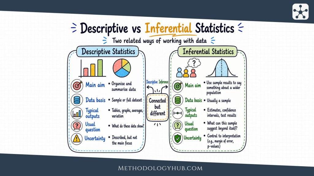
Statistical analysis is usually introduced through two broad types: descriptive statistical analysis and inferential statistical analysis. The distinction is useful because it separates two different claims a researcher may make from the same dataset. One claim stays close to the observations that were actually collected. The other uses those observations to say something careful about a wider population or process.

Descriptive and inferential analysis are best understood as two broad foundational categories rather than the only labels used in every field. Other terms, such as exploratory, predictive, causal, and prescriptive analysis, are also common, especially in applied research and data analytics. These labels usually describe the purpose of the analysis rather than a completely separate statistical category. For example, exploratory analysis often uses descriptive summaries, while predictive and causal analysis often rely on inferential models, assumptions, and study design.

In practice, the two types are rarely isolated. A researcher normally begins by describing the dataset, then moves into inference only when the sampling method, research question, and assumptions allow it. Without description, inference has no clear foundation. Without inference, many studies would stop at the sample and say nothing about the wider group the study was designed to examine.

Type	Main focus	Typical output
Descriptive statistical analysis	The data that were observed	Means, medians, percentages, standard deviations, tables, and graphs
Inferential statistical analysis	The population or process represented by the sample	Estimates, confidence intervals, p-values, test statistics, and model coefficients

The boundary between the two types is about the claim, not only the calculation. A mean can describe the average score in a sample. The same mean can also be used as a point estimate for a population average. In the first case, it is descriptive. In the second, it becomes part of inference.

Descriptive Statistical Analysis

Descriptive statistical analysis gives the first organised view of a dataset. It does not try to prove a hypothesis or estimate an unknown population value by itself. Its job is more basic and more necessary: it shows what the data look like before the researcher makes a wider claim.

A dataset can be difficult to read in its raw form. A table with hundreds of scores, measurements, or responses may contain a pattern, but that pattern is not always visible. Descriptive analysis turns those values into summaries that can be read, compared, and questioned. It tells the reader where the centre of the data lies, how much variation there is, which values are frequent, and whether the distribution has unusual features.

Measures of central tendency

Measures of central tendency describe the centre of a variable. The mean is the arithmetic average and is often useful when values are roughly balanced around a centre. The median is the middle value after the data are ordered, so it can be more informative when the distribution is skewed or contains extreme values. The mode identifies the most frequent value or category.

These measures are not interchangeable labels for the same idea. Suppose a set of completion times contains a few very slow values. The mean may increase because it is pulled by those long times, while the median may remain closer to the typical case. Reporting both can give the reader a clearer view than either one alone.

Measures of dispersion

Centre is only part of description. Two groups can have the same mean but very different amounts of variation. Measures of dispersion describe how spread out the values are. The range gives the distance between the smallest and largest value. The variance and standard deviation describe spread around the mean. The interquartile range focuses on the middle half of the data and is less affected by extreme values.

Frequencies, percentages, and distributions

When variables are categorical, descriptive analysis usually begins with counts and percentages. A survey response, diagnostic category, school type, or classification group cannot be averaged in the same way as a numerical score. Instead, the researcher reports how many observations fall into each category and what proportion of the sample each category represents.

For numerical variables, the distribution gives more detail than a single summary. A histogram can show whether values cluster around one peak, spread across a wide range, or lean strongly toward one side. A box plot can show the median, interquartile range, and possible outliers. A scatterplot can show whether two numerical variables appear to move together.

Descriptive analysis in the research sequence

Descriptive analysis usually appears before formal testing or modelling because it helps the researcher understand the conditions under which later results will be interpreted. It can reveal missing values, uneven group sizes, coding errors, or observations that need closer inspection. It can also show whether the planned method is reasonable for the shape and structure of the data.

This does not make descriptive analysis a preliminary chore. In many studies, the descriptive results are part of the findings themselves. A carefully written table of sample characteristics, a distribution of scores, or a comparison of group means can give readers the context they need to understand the rest of the analysis.

Inferential Statistical Analysis

Inferential statistics begins when the researcher uses sample data to make a reasoned statement about something beyond the observed cases. A study rarely measures every possible person, record, classroom, patient, organism, or measurement occasion. More often, it studies a sample and then asks what that sample suggests about a wider population or process.

This move from sample to population is useful, but it is never automatic. The researcher has to consider how the sample was selected, what population it can represent, how much sampling variation is expected, and whether the chosen method fits the data. Inferential statistical analysis gives this movement a formal structure.

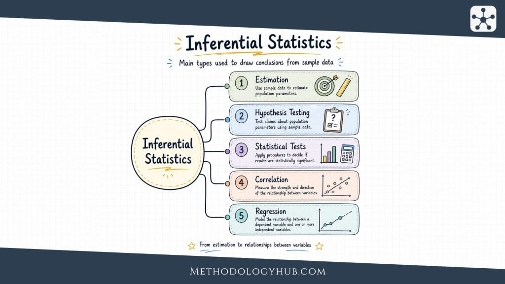
Estimation from sample data

One common form of inference is estimation. A sample mean can be used to estimate a population mean. A sample proportion can estimate a population proportion. A sample correlation can estimate a population correlation. The estimate gives the best available value from the data, but it should not be treated as exact.

For that reason, estimation is often reported with a confidence interval. A confidence interval places a range around the estimate. If a sample mean is 68 and the 95% confidence interval is 64 to 72, the interval gives a range of plausible values for the population mean under the method used. The width of the interval tells the reader something about precision. A narrow interval suggests less uncertainty than a wide one.

Hypothesis testing as inference

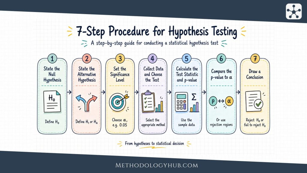
Another common form of inference is hypothesis testing. Here, the researcher begins with a null hypothesis, calculates a test statistic from the sample, and examines how unusual the result would be if the null hypothesis were true. The p-value helps with this judgement, while the significance level gives the rule for the statistical decision.

A test does not turn a sample result into certainty. It compares the observed result with what would be expected under a stated reference claim. If the result is difficult to reconcile with that claim, the researcher may reject the null hypothesis. If the result is not strong enough under the chosen rule, the researcher fails to reject it. Both outcomes still need interpretation in relation to sample size, effect size, design, and assumptions.

Sampling error and standard error

Sampling error is the difference between a sample statistic and the population parameter that occurs because only a sample was observed. It is not the same as a data collection error. Even a carefully selected random sample can differ from the population by chance.

The standard error describes the expected sample-to-sample variation of a statistic. A smaller standard error suggests a more precise estimate. A larger standard error suggests that repeated samples would tend to produce more spread in the estimate. Standard errors are central to confidence intervals and many hypothesis tests because they connect the observed result to expected sampling variation.

Assumptions and interpretation

Inferential methods depend on assumptions. These may concern independence of observations, sampling method, measurement level, distributional shape, equal variances, linearity, or expected cell counts. The exact assumptions depend on the method. A t-test, chi-square test, ANOVA, correlation, and regression model each asks different things of the data.

Assumptions do not make a study perfect. They state the conditions under which the method can be interpreted in the intended way. If the assumptions are not reasonable, the result may still appear in the software output, but the interpretation becomes weaker. This is why inferential statistical analysis should be read as a combination of design, calculation, and judgement.

The Statistical Analysis Process

Statistical analysis is often presented as if it starts when data are entered into software. In research, it starts earlier. The analysis is shaped by the research question, the design, the measurement choices, and the way data is collected. A good analysis therefore has a sequence, even when the work is not perfectly linear.

The sequence below shows how statistical analysis usually develops from a research question to a reported result. In practice, researchers often move back and forth. A preliminary graph may reveal a coding problem. A model assumption may send the researcher back to the data preparation stage. A result may require a clearer statement of the original question. That movement is part of analysis, not a failure of it.

Formulating the research question

The research question determines what the analysis is supposed to answer. A question about a difference between two independent groups points to a different analysis from a question about change within the same participants. A question about association between two numerical variables differs from a question about category counts.

At this stage, the researcher identifies the outcome variable, the explanatory variable if there is one, the unit of observation, and the population or setting to which the study refers. A clear question prevents the analysis from becoming a search through methods without direction.

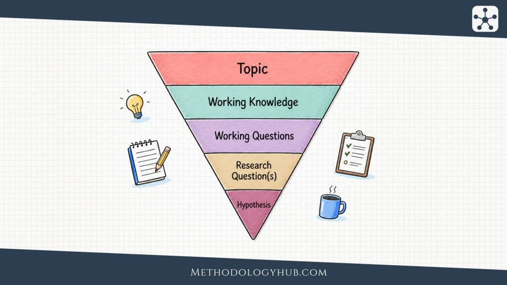
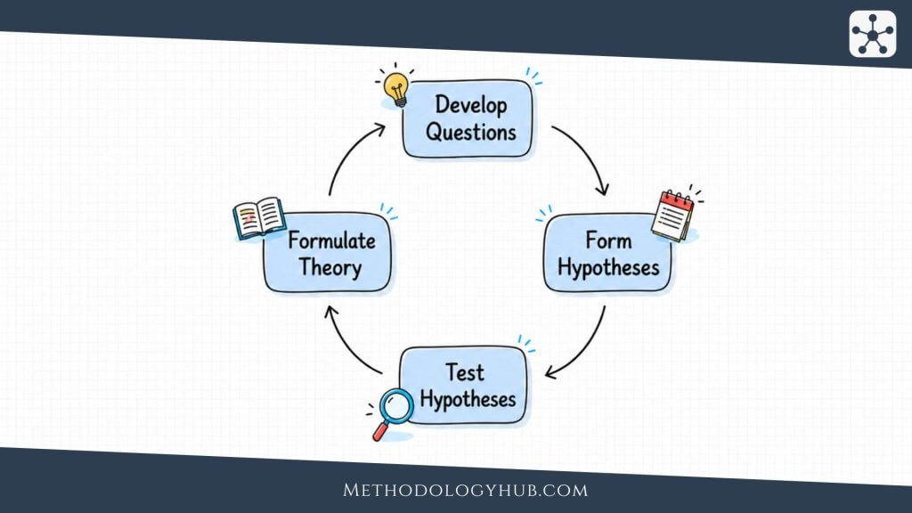
Developing hypotheses

Some studies express their research question as hypotheses. A hypothesis may state that two group means differ, that a population proportion is above a specified value, or that two variables are associated. In hypothesis testing, the null hypothesis gives the reference claim, while the alternative hypothesis states the pattern that would receive support if the evidence against the null is strong enough.

Not every analysis begins with formal hypotheses. Exploratory work may begin with a broad aim to describe patterns or examine possible relationships. Even then, the researcher should state what the analysis is intended to explore, otherwise the results can become hard to interpret.

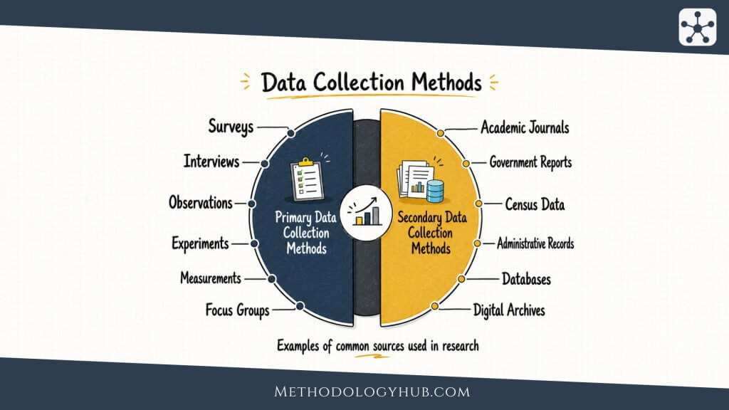
Collecting the data

Data collection links the research question to the observed values. The data may come from an experiment, survey, observational study, administrative record, laboratory measurement, archive, or secondary dataset. The method of collection affects what can later be claimed.

For example, random assignment in an experiment can support stronger causal interpretation than an observational comparison, while random sampling can support stronger population inference than a convenience sample. Statistical analysis cannot fully repair a weak design. It can only work with the evidence the design provides.

Preparing and cleaning the data

Data preparation is the part of statistical analysis that often receives less attention than it deserves. Before a test or model is run, the researcher needs to check whether variables are coded correctly, whether values fall within possible ranges, whether units are consistent, and whether missing values have been identified properly.

Consider a dataset with temperature measured in both Celsius and Fahrenheit, or a survey variable where missing answers have been coded as 99 but not labelled. If these details are missed, later calculations may be technically correct but substantively wrong. Data cleaning does not make the analysis more decorative. It makes the numbers interpretable.

Exploring and summarising the data

Initial exploration gives the researcher a first view of the dataset. This stage usually includes descriptive statistics, graphs, checks for missing values, group sizes, outliers, and distributional shape. The aim is not to force the data into a preferred method, but to understand what kind of data are actually present.

A histogram may show that a variable is highly skewed. A scatterplot may show a relationship that is curved rather than linear. A table may show that one group has far fewer observations than another. These details influence method choice and interpretation.

Selecting and applying the method

Statistical method selection brings the research question, data type, design, and assumptions together. A t-test, ANOVA, chi-square test, correlation, regression model, or nonparametric test may be appropriate in one setting and unsuitable in another. The same dataset can sometimes be analysed in more than one reasonable way, but the chosen approach should match the question being asked.

After a method is applied, the researcher reads the output. This may include estimates, standard errors, confidence intervals, test statistics, p-values, model fit indices, residual plots, or diagnostic checks. The output is not the interpretation itself. It is the material from which the interpretation is built.

Reporting the findings

Reporting statistical analysis means presenting the method and results clearly enough that a reader can understand what was done. Academic reporting usually includes the sample size, descriptive statistics, test or model used, relevant assumptions or checks, estimates, uncertainty measures, and a written interpretation tied to the research question.

A reader should be able to see whether the result describes the sample, estimates a population value, tests a hypothesis, or models a relationship. When tables, figures, and text tell the same story in different forms, the analysis becomes easier to read.

Types of Data in Statistical Analysis

The type of research data being analysed has a direct effect on method choice. A method designed for numerical measurements may not fit unordered categories. A method for independent observations may not fit repeated measurements from the same person. Before choosing a test, the researcher should understand how the variables are measured.

Numerical data

Numerical data express quantities. Examples include height, age, test score, reaction time, blood pressure, temperature, concentration, and number of errors. These variables can often be summarised with means and standard deviations, although the median and interquartile range may be more informative when the distribution is skewed.

Many common methods are designed for numerical outcomes. T-tests compare means in one or two groups. ANOVA compares means across three or more groups. Correlation and regression examine relationships between numerical variables. These methods can be useful, but they require attention to assumptions such as independence, approximate distributional shape, and variance patterns.

Categorical data

Categorical data place observations into groups. A variable might record field of study, diagnosis, region, response option, species, or presence versus absence of a condition. Since the values are categories rather than quantities, analysis often begins with counts and percentages.

When categorical variables are compared, cross-tabulations are often useful. A chi-square test of independence can examine whether two categorical variables are associated. If the outcome has two categories, logistic regression may be used to model the probability of one outcome category in relation to predictors.

Ordinal data

Ordinal data have ordered categories, but the distance between categories is not necessarily equal. Rating scales, severity levels, class ranks, and ordered response options often fall into this group. A response scale from strongly disagree to strongly agree has an order, but the distance from one category to the next may not be measurable in the same way as centimetres or seconds.

Ordinal variables are often summarised with medians, percentages, or distribution tables. Rank-based methods can be useful when the order is meaningful but the assumptions of numerical methods are not appropriate. In some research settings, scale totals with many ordered items are treated as approximately numerical, but that choice should be explained rather than assumed silently.

Repeated and time-based data

Some datasets contain repeated observations. A patient may be measured at several clinic visits. A student may take a test at the beginning and end of a course. A sensor may record values every hour. These observations are usually related to one another, so methods that assume complete independence may not be suitable.

Repeated and time-based data often require methods that recognise the structure of measurement. Paired tests, repeated-measures procedures, mixed models, and time series methods are examples. Simple line graphs can also be useful at the descriptive stage because they show change over time in a way that a single average cannot.

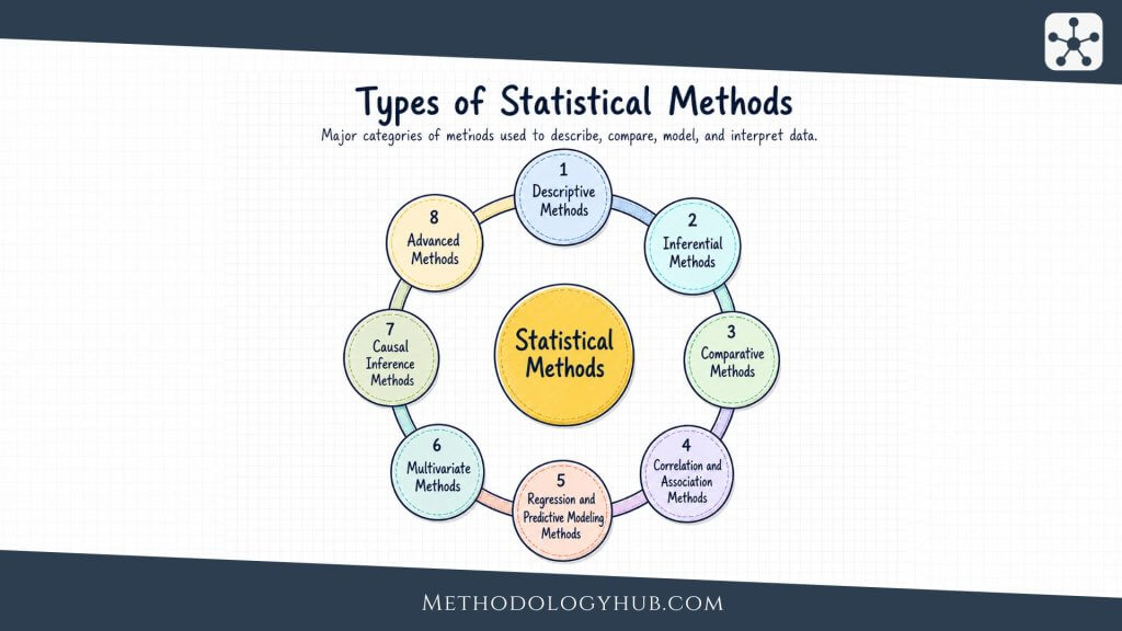
Methods Used in Statistical Analysis

Statistical analysis includes many methods, but several appear frequently in introductory research courses, dissertations, journal articles, and laboratory reports. The methods below are not a complete catalogue. They are a practical map of procedures that students and researchers often meet early.

Summary measures

Summary measures condense a dataset into interpretable numbers. The mean gives the arithmetic average, while the median gives the middle value when observations are ordered. The mode identifies the most frequent value or category. Measures of spread, such as range, variance, standard deviation, and interquartile range, show how much variation exists around a centre.

These measures are simple, but they are not trivial. A mean without a standard deviation can hide large variation. A mean in a strongly skewed distribution can be less representative than the median. A percentage can look precise while being based on a very small number of cases. Summary measures should be read with the data structure in view.

Hypothesis testing

Hypothesis testing is a common method for evaluating a statistical claim with sample data. It begins with a null hypothesis, which gives the reference claim, and an alternative hypothesis, which states the pattern that would receive support if the evidence against the null is strong enough. The analysis then calculates a test statistic and p-value from the sample.

This method appears inside many familiar tests rather than beside them as a completely separate tool. A t-test, ANOVA, chi-square test, correlation test, or regression coefficient test can all be used for hypothesis testing. The procedure gives the researcher a decision rule, but the result should still be read with descriptive statistics, effect size, confidence intervals, and the research design in view.

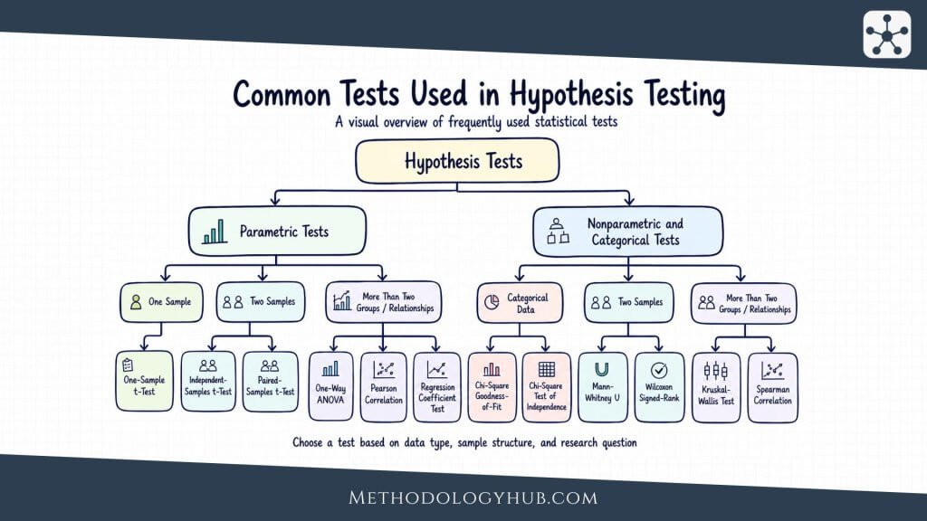
T-tests

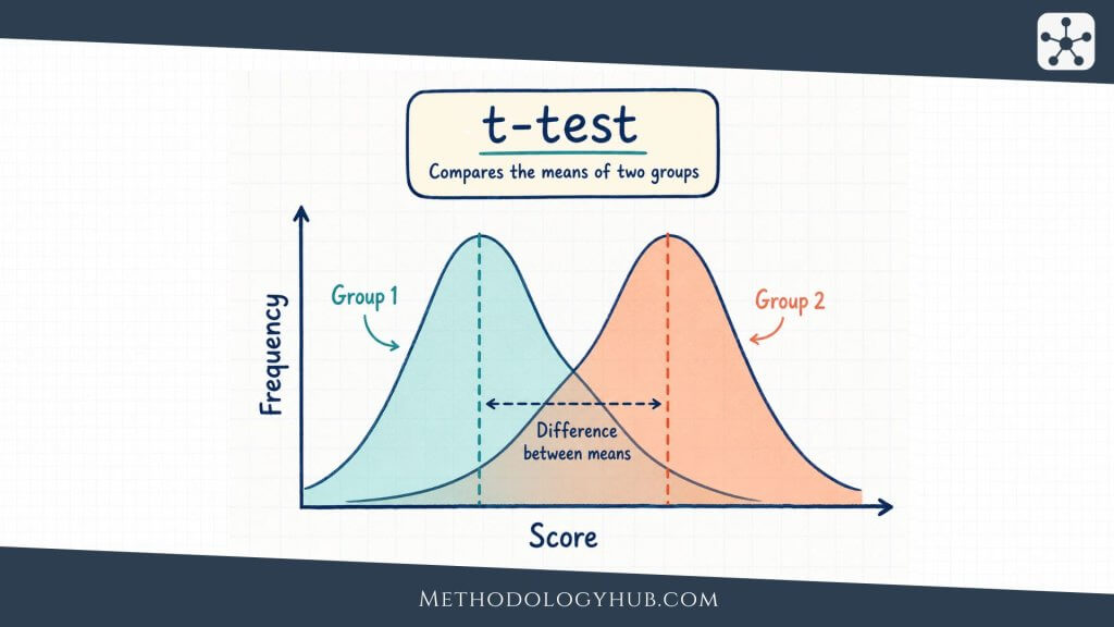
A t-test is used when the analysis focuses on a mean and the outcome is numerical. A one-sample t-test compares a sample mean with a specified value. An independent-samples t-test compares the means of two separate groups. A paired-samples t-test compares two related measurements, such as before and after scores from the same participants.

For example, an education researcher might compare reading scores from two independent classes. If the outcome is numerical and the assumptions are reasonable, an independent-samples t-test can examine whether the observed difference between means is larger than expected under a no-difference reference claim.

ANOVA (Analysis of variance)

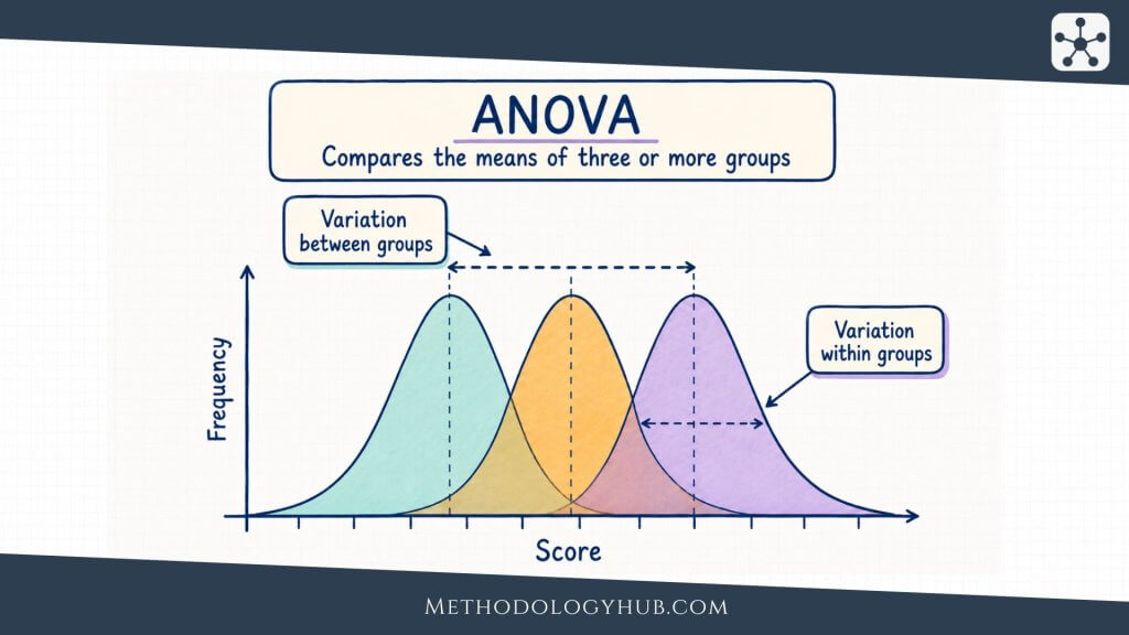
Analysis of variance, usually called ANOVA, is used when a researcher compares means across three or more groups. Instead of running many separate t-tests, ANOVA compares variation between groups with variation within groups. The result is expressed with an F statistic and a p-value.

If the ANOVA result suggests that not all group means are equal, follow-up comparisons may be used to examine which groups differ. The interpretation should include descriptive statistics as well. ANOVA can indicate that a difference exists somewhere among the groups, but the group means and intervals help the reader understand the pattern.

Chi-square tests

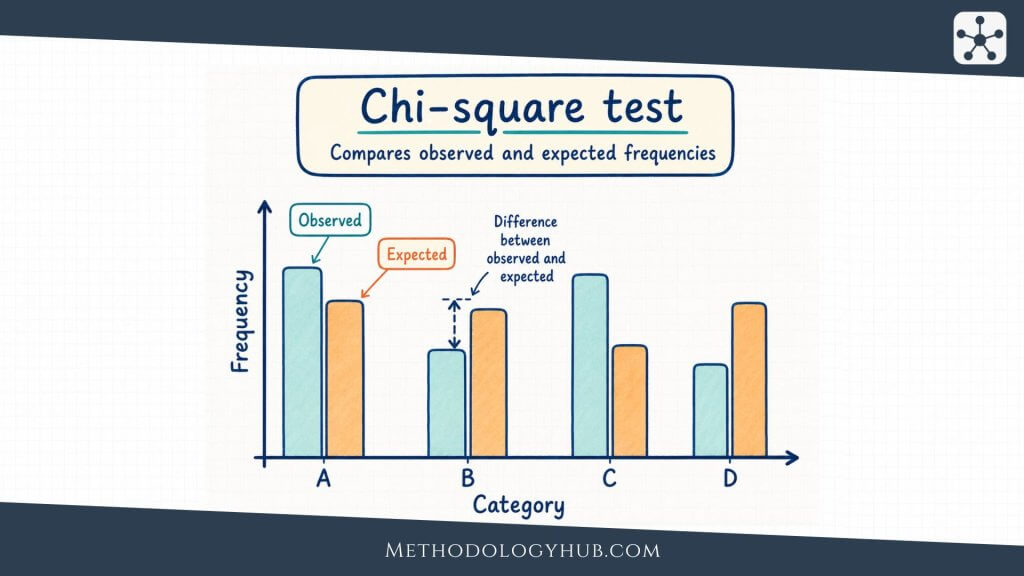
Chi-square tests are used with categorical counts. A chi-square goodness-of-fit test compares observed counts with expected counts for one categorical variable. A chi-square test of independence examines whether two categorical variables are associated in a contingency table.

In a biology teaching study, a researcher might compare observed trait counts with expected genetic ratios. In a social science survey, a researcher might examine whether preferred study location is associated with year level. Both examples use counts in categories rather than numerical means.

Correlation analysis

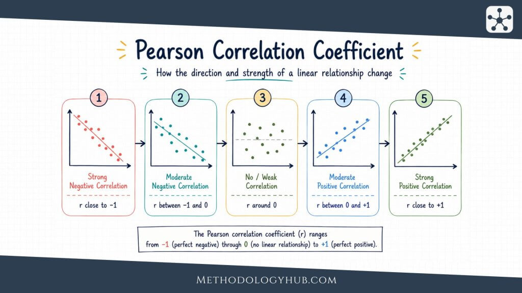
Correlation analysis examines the direction and strength of association between two variables. Pearson’s correlation coefficient, often written as r, is used for linear association between two numerical variables. It ranges from -1 to +1. A positive value means higher values of one variable tend to appear with higher values of the other. A negative value means higher values of one variable tend to appear with lower values of the other.

Correlation can be descriptive or inferential. A sample correlation describes the association in the observed data. A hypothesis test or confidence interval for the correlation uses the sample to make a statement about a population relationship. In either case, correlation does not by itself show that one variable caused the other to change.

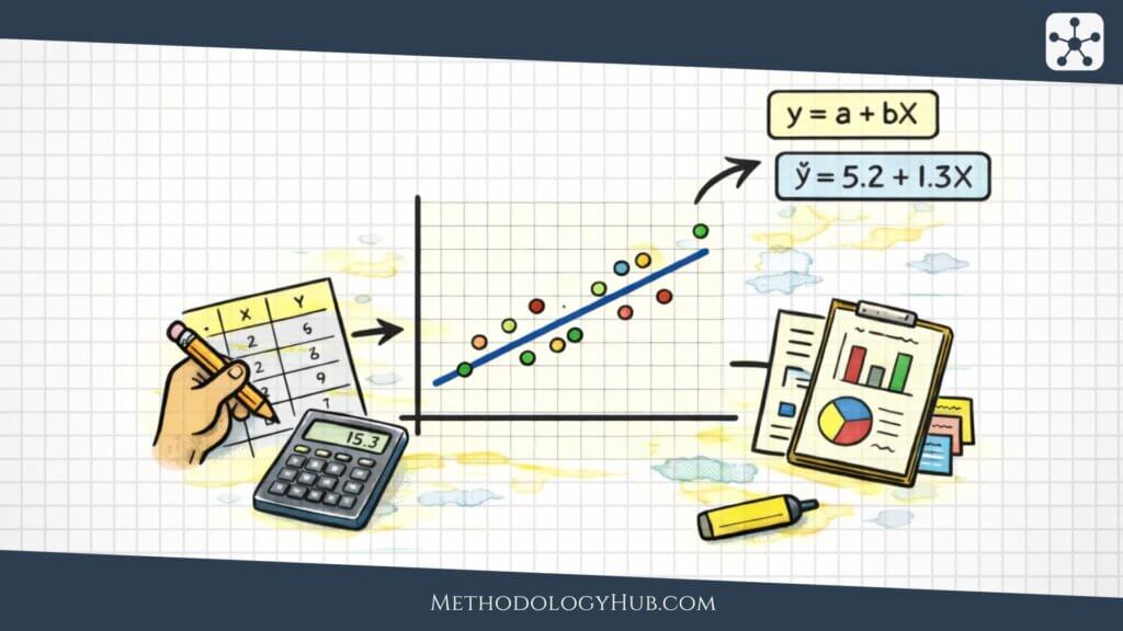
Regression analysis

Regression analysis models an outcome variable using one or more predictor variables. In simple linear regression, there is one predictor and one outcome. In multiple regression, several predictors are included in the same model. The model estimates how the outcome changes as predictors change, under the conditions specified by the model.

Regression is often used when a researcher wants to examine relationships while accounting for more than one predictor. For example, a study of academic performance might model final score using study time, prior score, and attendance. Each coefficient has to be interpreted in relation to the variables included in the model, the measurement scale, and the study design.

Nonparametric methods

Nonparametric methods are often used when the assumptions of common parametric methods are not suitable, or when the data are ordinal. The Mann-Whitney U test can compare two independent groups using ranks. The Wilcoxon signed-rank test can be used for paired observations. The Kruskal-Wallis test can compare three or more independent groups using ranks.

These methods should not be treated as automatic replacements whenever a preferred test is inconvenient. They often answer slightly different questions. The researcher should choose them because they fit the measurement level, distribution, or design of the data.

Interpreting Statistical Results

Interpretation is where statistical analysis becomes more than calculation. A software output may show a p-value, confidence interval, coefficient, standard error, or model summary. The researcher still has to decide what the result says about the research question and what it does not say.

A careful interpretation keeps several pieces together: the size of the result, the uncertainty around it, the assumptions of the method, the quality of the measurements, and the study design. No single number can carry all of that information.

Statistical significance

Statistical significance is a decision made in hypothesis testing. If the p-value is less than or equal to the chosen significance level, often 0.05, the null hypothesis is rejected under that rule. A statistically significant result suggests that the observed data would be unusual if the null hypothesis and model assumptions were true.

This wording is deliberate. A p-value does not give the probability that the null hypothesis is true. It also does not measure the size of the result. A very small difference can be statistically significant in a very large sample, while a larger difference may be uncertain in a small sample. For this reason, statistical significance should usually be read with effect size and confidence intervals.

Effect size

Effect size describes the magnitude of a result. In a comparison of two means, an effect size may express the difference in standard deviation units. In correlation, the coefficient itself shows direction and strength of linear association. In regression, coefficients estimate the expected change in the outcome for a change in the predictor, while other included predictors remain in the model.

Effect size helps the reader move beyond a yes-or-no decision. Two studies can have similar p-values but different magnitudes. They can also have similar magnitudes but different p-values because of sample size or variability. Reporting effect size makes the result more interpretable.

Confidence intervals

A confidence interval gives a range of plausible values for a population parameter, based on the sample and the method used. A 95% confidence interval for a mean difference might range from 1.2 to 5.8 points. That interval gives more information than the point estimate alone because it shows both direction and precision.

Wide intervals suggest greater uncertainty. Narrow intervals suggest more precision. If an interval for a difference crosses zero, the result is less clear under that analysis. If the entire interval lies above or below zero, the direction of the estimated difference is clearer, although interpretation still depends on design and assumptions.

Assumptions and model fit

Statistical methods rely on assumptions. These may involve independence of observations, the level of measurement, distributional shape, equal variances, linearity, or the structure of residuals. A result can be calculated even when assumptions are poor, but the interpretation may then be weak.

Assumption checks should be connected to the method. For regression, residual plots can help detect nonlinearity, unequal variance, or unusual observations. For chi-square tests, expected cell counts should be checked. For repeated measurements, the dependence among observations should be recognised. These checks help the researcher decide how much confidence to place in the result.

Association and causation

Many statistical analyses examine associations. Correlation may show that two variables tend to vary together. Regression may show that a predictor is associated with an outcome after other predictors are included. These results do not automatically show causation.

Causal interpretation depends on design, timing, measurement, possible confounding variables, and theoretical reasoning. Randomised experiments can support stronger causal claims than observational studies, but even experiments require careful interpretation. Statistical analysis can provide evidence about patterns in data. The research design determines how far those patterns can be interpreted.

Examples of Statistical Analysis

Statistical analysis appears across academic fields, although the data and questions differ. A medical trial, a classroom study, a public health survey, a psychology experiment, and a laboratory comparison may use different designs, but each needs a transparent connection between question, data, method, and interpretation.

Medicine and clinical research

In medicine, statistical analysis is used to compare treatments, estimate risk, examine diagnostic accuracy, and analyse patient outcomes. Clinical trials often compare groups that receive different interventions. Observational studies may examine associations between exposures and outcomes while accounting for other variables.

Medical results are usually read with close attention to confidence intervals, effect sizes, adverse event counts, and sample selection. A statistically significant treatment difference may still need careful interpretation if the interval is wide, the sample is narrow, or the outcome is measured over a short period.

Public health and epidemiology

Public health research often works with rates, proportions, risk estimates, surveillance data, and population-level patterns. Statistical analysis may be used to estimate disease prevalence, compare incidence across groups, evaluate screening data, or model changes over time.

Because public health data often come from large and complex populations, sampling, missing data, measurement definitions, and confounding variables require careful treatment. A pattern in a population dataset can be informative, but it must still be read in relation to how the data were collected.

Education and psychology

Education and psychology frequently analyse test scores, survey scales, behavioural measures, reaction times, ratings, and repeated measurements. A researcher may compare groups, examine pre-test and post-test change, estimate reliability, or model relationships between predictors and outcomes.

In these fields, measurement quality is especially visible. A score or scale total is not only a number. It is the result of an instrument, a response process, and a scoring rule. Statistical analysis should therefore be interpreted alongside the way the variable was measured.

Social sciences

In sociology, political science, communication studies, and related fields, statistical analysis often uses survey data, administrative records, experiments, and longitudinal datasets. Researchers may examine group differences, attitudes, demographic patterns, institutional outcomes, or changes over time.

Social science data often involve nested or clustered observations, such as students within schools or individuals within regions. In those settings, the structure of the data may require methods that account for clustering rather than treating all observations as fully independent.

Natural sciences and laboratory research

Laboratory and natural science research may analyse measurements from experiments, field samples, instruments, repeated trials, or controlled comparisons. Statistical analysis can help summarise variation, compare conditions, estimate measurement precision, and model relationships among variables.

In a laboratory setting, repeated measurements and calibration procedures are often central. A small difference between conditions may be interpreted differently depending on measurement precision, replication, and the stability of the experimental procedure.

Statistical Analysis Tools

Statistical analysis can be carried out by hand for small examples, but research datasets are usually analysed with software. The tool should not replace statistical reasoning. It should help the researcher organise data, apply suitable methods, check results, and report analysis transparently.

R

R is widely used in academic research for statistical modelling, graphics, simulation, and reproducible workflows. It has packages for descriptive statistics, regression, mixed models, survival analysis, Bayesian analysis, data visualisation, and many specialised methods. Because code can be saved and rerun, R is useful when transparency and reproducibility are needed.

Python

Python is used for data preparation, numerical computation, statistical modelling, and machine learning. Libraries such as pandas, NumPy, SciPy, statsmodels, matplotlib, and scikit-learn support many parts of the analysis process. Python is often useful when statistical analysis is combined with data processing, simulation, or larger computational workflows.

SPSS

SPSS is common in social science, education, psychology, and health-related teaching contexts. It uses menus for many statistical procedures, which can make it approachable for students and researchers who are not yet comfortable with code. It can also produce syntax files, which are useful because they preserve the steps used in an analysis.

SAS

SAS is widely used in clinical research, epidemiology, and large institutional settings where structured data management and regulatory compliance are important. It provides tools for data handling, advanced statistical modelling, and reporting. SAS programs can be saved and reused, which supports consistency, documentation, and reproducibility in research workflows.

Stata

Stata is commonly used in social science, economics, public health, and policy-oriented research. It offers a wide range of statistical methods, including regression, panel data analysis, time-series analysis, and survey methods. Stata uses a command-based interface, and analyses can be saved as scripts, making it easier to review, share, and reproduce results.

MATLAB

MATLAB is used for numerical computation, simulation, and data analysis in engineering, physics, and applied mathematics. It includes toolboxes for statistics, machine learning, and signal processing. MATLAB is especially useful when statistical analysis is combined with mathematical modelling or algorithm development.

Minitab

Minitab is commonly used in education and industry, particularly in quality improvement and Six Sigma projects. It provides a user-friendly interface for statistical analysis, including descriptive statistics, hypothesis testing, regression, and design of experiments. Minitab is often chosen when ease of use and clear graphical output are important.

Spreadsheet software

Spreadsheet software can be useful for simple data entry, basic descriptive summaries, and teaching examples. It is less suitable for complex analyses, large datasets, or workflows that require detailed reproducibility. A spreadsheet can hide formulas, make accidental changes easy, and make it difficult to trace every step of the analysis.

Reproducible analysis

Reproducibility means that the analysis can be checked, repeated, and understood by another reader or by the same researcher later. Script-based tools help because the commands show how data were cleaned, transformed, summarised, and analysed. Reports created from code can also reduce the risk of copying a number incorrectly from one file to another.

Even when menu-based software is used, researchers can improve transparency by saving syntax, documenting variable coding, keeping a data dictionary, recording exclusion rules, and separating raw data from cleaned data. These habits make the final statistical analysis easier to review.

Conclusion

Statistical analysis gives researchers a structured way to work with quantitative data. It begins with a research question, continues through data collection and preparation, and then uses descriptive summaries, inferential procedures, and statistical models to examine patterns in the data.

The main ideas are connected. Descriptive statistics show what was observed. Inferential statistics use sample data to estimate, test, and model beyond the sample. Data type guides method choice. Assumptions shape interpretation. P-values, effect sizes, confidence intervals, and model diagnostics each tell part of the story.

A strong analysis is careful rather than automatic. It does not treat software output as a conclusion by itself. It reads results in relation to the research design, the variables, the sample, the measurement process, and the uncertainty surrounding the estimate. When these parts are kept together, statistical analysis becomes a disciplined way of reasoning from numerical evidence.