Chi-square test is a statistical test used to analyse categorical data. It helps researchers compare observed counts with expected counts, either to see whether one categorical variable follows an expected pattern or to examine whether two categorical variables are associated.
This article explains what the chi-square test is, how the chi-square statistic is calculated, which assumptions need attention, when to use the test, how to work through an example, and how to interpret and report the result in academic writing.
What Is the Chi-Square Test?
The chi-square test is a method in inferential statistics for analysing counts in categories. Instead of comparing means, as a t-test or ANOVA would do, it compares how many cases fall into categories with how many cases would be expected under a stated null hypothesis.
Suppose a school asks 120 students which of three study spaces they usually use: library, classroom, or home. If the researcher expects students to choose the three options equally often, the chi-square test can compare the observed counts with that equal-distribution expectation. In another study, the researcher may ask whether preferred study space is associated with year level. In that case, the counts are placed in a table, and the test compares the observed table with the table expected if the two variables were independent.
Chi-square test definition
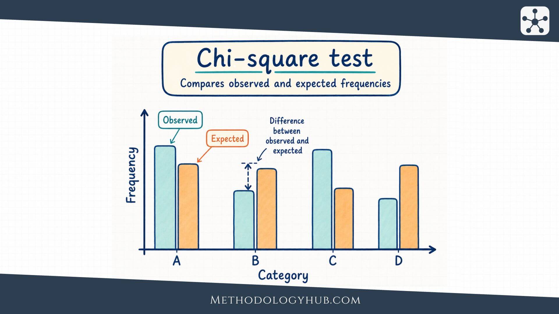
The chi-square test is a statistical test that compares observed frequencies with expected frequencies. The observed frequencies are the counts actually found in the data. The expected frequencies are the counts predicted by the null hypothesis. The larger the overall gap between observed and expected counts, relative to the expected counts, the larger the chi-square statistic becomes.
The test is most often used with nominal or ordinal categories, such as response option, group membership, school type, diagnosis category, voting preference, or outcome status. A chi-square test does not analyse raw scale scores, averages, or continuous measurements directly. If the research question is about mean test scores, reaction times, heights, or scale totals, another method will usually fit better.

The basic idea behind the test
The logic of the chi-square test is easier to follow when the expected counts are treated as a reference pattern. The null hypothesis describes what the counts should look like if there is no difference from an expected distribution, or if two categorical variables are unrelated. The sample gives the observed counts. The test asks whether the observed pattern is far enough from the expected pattern to be difficult to explain as ordinary sample variation.
This does not mean that every visible difference is statistically persuasive. Counts almost never match expected values perfectly. A class may have 38 students choosing one option and 42 choosing another even when there is no real preference in the wider population. The chi-square test helps judge whether the differences are small enough to treat as ordinary variation or large enough to reject the null hypothesis under the chosen significance level.
Observed and expected frequencies
Observed frequencies come directly from the dataset. If 27 students selected library, 41 selected classroom, and 52 selected home, those three numbers are observed frequencies. They are usually written as O in the formula.
Expected frequencies are calculated from the null hypothesis. In a goodness-of-fit test with three equally likely categories and 120 students, each category would have an expected count of 40. In a test of independence, the expected count in each cell is calculated from the row total, column total, and overall total. That calculation shows what the table would look like if the two variables were independent while keeping the same margins.
Chi-square test as part of hypothesis testing
The chi-square test follows the usual structure of hypothesis testing. The researcher states a null hypothesis, states an alternative hypothesis, chooses a significance level, calculates a test statistic, finds a p-value, and then interprets the result in relation to the research question.
For a goodness-of-fit test, the null hypothesis may state that the population follows a particular distribution across categories. For a test of independence, the null hypothesis states that the two categorical variables are independent in the population. The alternative hypothesis then states that the distribution differs from the expected pattern, or that the two variables are associated.
Key Aspects of the Chi-Square Test
The chi-square test becomes much less mysterious once its main parts are seen as one connected process. A researcher begins with a categorical research question, organises the data into counts, calculates the expected counts under the null hypothesis, and then measures the overall distance between the observed and expected patterns.
These parts are not separate vocabulary items to memorise. They are steps in the same comparison. The observed table shows what happened in the sample. The expected table shows what the null hypothesis predicts. The chi-square statistic measures the gap between them. Degrees of freedom identify the relevant chi-square distribution. The p-value then places the statistic in that distribution.
Categorical variables
A chi-square test is used when the data are counts in categories. The categories may have no natural order, as with subject area, school type, or response choice. They may also have an order, as with low, medium, and high preference ratings, as long as the analysis treats them as categories rather than as numerical scores.
This distinction affects test selection. If a researcher records whether students passed or failed an exam, the outcome is categorical. If the researcher records the actual exam score from 0 to 100, the outcome is numerical. A pass-or-fail table may be analysed with a chi-square test. A comparison of mean scores would usually call for a t-test, ANOVA, or another method for numerical outcomes.
Counts, not percentages alone
Percentages are helpful for interpretation, but the chi-square test itself uses counts. A table that says 60% of one group passed and 45% of another group passed is easier to read than raw counts alone, but the test needs the actual number of people in each cell. A difference between 60% and 45% means something different when it is based on 20 people than when it is based on 2,000 people.
For this reason, reports should usually show both counts and percentages. Counts let the reader see the amount of data behind the analysis. Percentages help the reader understand the direction and size of the pattern.
The chi-square statistic
The chi-square statistic is usually written as χ2. It is calculated by comparing each observed count with its expected count, squaring the difference, dividing by the expected count, and adding those values across all categories or cells.
A cell with a large gap between observed and expected values contributes more to the statistic than a cell with a small gap. The division by the expected count is also important. A difference of 5 cases is more noticeable when 10 were expected than when 500 were expected. The formula therefore considers both the size of the difference and the scale of the expected count.
Degrees of freedom
Degrees of freedom connect the calculated statistic to the correct chi-square distribution. In a goodness-of-fit test, degrees of freedom are usually the number of categories minus 1, with further adjustments if parameters were estimated from the data. In a test of independence, degrees of freedom are calculated from the number of rows and columns in the table.
Degrees of freedom for independence: df = (number of rows – 1) x (number of columns – 1)
For example, a table with 3 teaching methods and 2 outcome categories has 3 rows and 2 columns. The degrees of freedom are (3 – 1) x (2 – 1), which gives 2. The p-value is then found by comparing the calculated χ2 value with a chi-square distribution with 2 degrees of freedom.
p-value and significance level
The p-value shows how unusual the observed pattern would be if the null hypothesis were true and the test assumptions were satisfied. A small p-value means the observed counts are relatively far from what the null hypothesis predicts. If the p-value is less than or equal to the chosen significance level, often 0.05, the researcher rejects the null hypothesis.
The p-value does not tell the probability that the null hypothesis is true. It also does not tell the size of the association. A very large sample can produce a small p-value for a pattern that is not very large in practical terms. That is why interpretation should include the actual table, percentages, and an effect size when possible.
Effect size for chi-square tests
For a chi-square test of independence, Cramer’s V is a common effect size. It ranges from 0 upward, with 0 meaning no association in the sample table. Larger values show stronger association, although the meaning of small, medium, or large depends on the field, table size, and research context.
For a 2 x 2 table, the phi coefficient can also be used. In larger contingency tables, Cramer’s V is usually easier to report because it adjusts for the table dimensions. The effect size helps the reader move beyond the yes-or-no decision of statistical significance.
Types of Chi-Square Tests
The term chi-square test is used for more than one testing situation. In introductory research methods and statistics courses, two forms appear most often: the chi-square goodness-of-fit test and the chi-square test of independence. Both use observed and expected counts, but they answer different questions.
The easiest way to separate them is to look at the number of categorical variables. A goodness-of-fit test usually works with one categorical variable. A test of independence works with two categorical variables arranged in a contingency table.
Chi-square goodness-of-fit test
A chi-square goodness-of-fit test checks whether the distribution of one categorical variable matches an expected distribution. The expected distribution may be equal across categories, based on theory, based on a known population distribution, or based on a model specified before the test.
For example, a researcher may test whether students choose four essay topics equally often. If 200 students choose from four topics and the null hypothesis says each topic is equally likely, the expected count is 50 for each topic. The test compares the observed topic counts with those expected counts.
Chi-square test of independence
A chi-square test of independence examines whether two categorical variables are associated. The data are arranged in a table, with one variable forming the rows and the other forming the columns. The test compares the observed count in each cell with the count expected if the two variables were independent.
For example, a researcher may examine whether teaching method is associated with pass or fail status. Teaching method has categories such as lecture, seminar, and mixed format. Outcome has categories such as pass and fail. The test asks whether the pass-fail distribution looks similar across teaching methods or whether the observed table departs from independence.
Chi-square test of homogeneity
The test of homogeneity is closely related to the test of independence. It compares the distribution of a categorical outcome across two or more groups. The calculations are the same as the chi-square test of independence, but the research design is often described differently.
For example, a researcher may sample three schools separately and compare the distribution of preferred feedback format across those schools. The question is whether the category distribution is homogeneous across groups. In many introductory settings, this is taught together with the test of independence because the table, formula, degrees of freedom, and p-value calculation are the same.
| Type of chi-square test | Typical question | Data structure |
|---|---|---|
| Goodness-of-fit test | Does one categorical variable follow an expected distribution? | One categorical variable with observed and expected counts |
| Test of independence | Are two categorical variables associated? | Two categorical variables in a contingency table |
| Test of homogeneity | Do several groups have the same distribution across categories? | A categorical outcome compared across groups |
Pearson chi-square and related tests
When people say chi-square test in an introductory setting, they usually mean Pearson’s chi-square test. It is the standard test based on the familiar sum of squared differences between observed and expected counts divided by expected counts.
Related methods include Fisher’s exact test for small 2 x 2 tables, the likelihood-ratio chi-square test in software output, and McNemar’s test for paired nominal data.
Assumptions
The chi-square test has fewer distributional assumptions than many tests for numerical data, but it still depends on conditions that should be checked. The assumptions are mostly about how the data were collected, how categories were formed, and whether expected counts are large enough for the chi-square approximation to work well.
These assumptions should be considered before the result is interpreted. A table can always be produced by software, but a calculated p-value is only useful when the method fits the data and research design.
Categorical data
The variables in a chi-square test should be categorical. Each observation must be placed into one category for the variable being analysed. In a test of independence, each observation is classified on both categorical variables, such as teaching method and pass-fail outcome.
Problems occur when numerical data are forced into categories without a clear reason. For example, converting a detailed exam score into high and low groups may lose information. Sometimes categories are necessary for the research question, but the choice should be explained rather than treated as automatic.
Independent observations
The observations should be independent. One person’s category should not determine or duplicate another person’s category. If the same student appears twice in the table, or if several observations come from the same family, classroom, clinic, or matched pair, the ordinary chi-square test may overstate the amount of independent information in the data.
Independence is about the design, not only the table. A table may look ordinary even when observations are clustered or repeated. When the design is paired, repeated, or nested, the researcher should consider a method designed for that structure.
Mutually exclusive categories
Categories should be mutually exclusive. Each observation should fit into one category per variable. If a participant can choose more than one response option, the resulting counts may not be suitable for an ordinary chi-square table unless the analysis is designed for multiple-response data.
For example, a survey question that asks students to select all study resources they use creates overlapping categories. One student may select videos, textbooks, and peer discussion. Treating those choices as if they came from separate independent people would distort the analysis.
Expected cell counts
The chi-square test uses an approximation that works better when expected counts are not too small. A common introductory rule says that expected counts should generally be at least 5 in each cell, or at least that no more than a small proportion of cells have expected counts below 5 and none are extremely small. Different textbooks and fields phrase this rule with slight variations.
The important point is that small expected counts can make the p-value less reliable. If expected counts are too low, the researcher may combine categories when that is conceptually sensible, use Fisher’s exact test for a small 2 x 2 table, or choose another method for categorical data.
A suitable sample size
Sample size affects both the assumptions and the interpretation. If the sample is too small, expected counts may be too low. If the sample is very large, even a small difference between observed and expected counts may become statistically significant. Neither situation should be handled mechanically.
In a small study, a non-significant chi-square test may simply have too little information to detect a pattern. In a very large study, a significant result may need careful effect-size interpretation. The table itself remains important because it shows where the differences occur and how large they are in ordinary percentage terms.
Random sampling or suitable design
When the goal is to generalise from a sample to a population, the sampling method should support that claim. A chi-square p-value does not repair a biased or poorly defined sample. If the data come from a convenience sample, the analysis may still describe the sample and test patterns within it, but wider population claims should be cautious.
This connects the chi-square test to broader issues in sampling and data collection methods. The statistical test is only one part of the research design.
When to Use the Chi-Square Test
Use the chi-square test when the research question is about frequencies in categories. The question may focus on whether one categorical variable follows an expected distribution, or whether two categorical variables are associated. The test is especially common in education, psychology, sociology, public health, biology, and other fields where researchers collect category counts.
The decision begins with the structure of the data. If the outcome is a count in categories, the chi-square test may be suitable. If the outcome is a numerical score, the researcher should usually look at tests for means, relationships, or models designed for numerical data.
Use it for one categorical variable and an expected pattern
A goodness-of-fit test fits when the researcher has one categorical variable and a clear expected distribution. The expected distribution should be chosen before looking at the data. It may come from a theory, a prior population distribution, an equal distribution, or a stated model.
For example, a teacher may want to know whether students choose four project formats equally often. A genetics example may compare observed trait counts with expected Mendelian ratios. A survey researcher may compare the sample distribution of age categories with a known population distribution.
Use it for two categorical variables in a table
A test of independence fits when both variables are categorical and the researcher wants to examine association. The table may compare school type and extracurricular participation, treatment group and recovery status, teaching method and pass-fail outcome, or age category and preferred learning resource.
The test does not say that one variable caused the other. It evaluates whether the observed table differs from what would be expected if the variables were independent. Causal interpretation still depends on the design, measurement, timing, and possible alternative explanations.
Use another test when the outcome is numerical
If the research question compares average scores, the chi-square test is usually not the right tool. A two-group mean comparison may call for a t-test. A comparison of three or more group means may call for ANOVA. A question about the linear relationship between two numerical variables may call for correlation tests or regression tests.
There are situations where numerical data are grouped into categories for a specific reason, but this should not be done only to make a chi-square test possible. Categorising a numerical variable can remove detail and reduce statistical information.
Use a different method for ranked or paired data when needed
Some research questions involve ordinal scores, ranks, or paired observations. If two independent groups are compared on an ordinal outcome, the Mann-Whitney U test may be more suitable than turning the data into categories. If the same participants are classified before and after an intervention, McNemar’s test may fit better than an ordinary chi-square test of independence.
For relationships between ranked variables, methods such as Spearman’s rank correlation or Kendall’s tau may be better aligned with the data structure.
| Research situation | Typical choice | Reason |
|---|---|---|
| One categorical variable compared with expected proportions | Chi-square goodness-of-fit test | The question concerns a category distribution |
| Two categorical variables in a contingency table | Chi-square test of independence | The question concerns association between categories |
| Two independent group means | t-test | The outcome is numerical |
| Three or more group means | ANOVA | The comparison is about means, not counts |
| Two numerical variables | Correlation or regression | The question concerns numerical association or prediction |
Formula for the Chi-Square Test
The chi-square formula compares each observed count with its expected count. It does this one category or cell at a time, then adds the pieces together. The formula looks compact, but each part has a direct meaning.
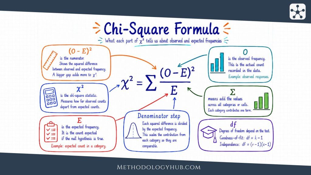
In this formula, O is the observed frequency, E is the expected frequency, and Σ means that the values are added across all categories or cells. The subtraction O – E measures the difference between observed and expected counts. Squaring the difference removes negative signs and gives larger differences more weight. Dividing by E scales the difference by the expected count.
Formula in words
A plain way to read the formula is this: for every category or table cell, find how far the observed count is from the expected count, square that distance, divide by the expected count, and then add the results. The final value is the chi-square statistic.
When observed and expected counts are close, the contributions are small and the statistic stays low. When several cells have observed counts far from expected counts, the statistic becomes larger. The p-value then tells how unusual that statistic is under the relevant chi-square distribution.
Expected counts in a goodness-of-fit test
In a goodness-of-fit test, expected counts come from the expected proportions. If the expected proportions are equal, the calculation is simple. With 120 observations and 3 categories, equal proportions give 40 expected observations per category.
If expected proportions are not equal, each expected count is found by multiplying the total sample size by the expected proportion for that category. For example, if a population distribution is expected to be 50%, 30%, and 20% across three categories, a sample size of 200 would give expected counts of 100, 60, and 40.
Expected counts in a test of independence
In a test of independence, expected counts are calculated from the margins of the table. Each expected cell count uses the row total, the column total, and the grand total.
Expected cell count: E = (row total x column total) / grand total
This formula gives the count that would be expected in a cell if the two variables were independent. For example, if 40 students are in a teaching-method row, 75 students passed overall, and 120 students are in the whole table, the expected number of passing students in that row is 40 x 75 / 120, which equals 25.
From statistic to p-value
After the chi-square statistic is calculated, it is compared with a chi-square distribution using the appropriate degrees of freedom. Statistical software usually reports the p-value directly. In hand calculations, a chi-square table may be used to compare the statistic with a critical value.
The p-value gives the probability of a chi-square statistic at least as large as the observed one, assuming the null hypothesis is true. A large statistic usually gives a smaller p-value because the observed counts are farther from what the null hypothesis predicts.
Example Usage
A worked example shows how the chi-square test moves from a research question to a table, then from the table to a statistical result. The numbers below are small enough to follow by hand, but the same logic applies when statistical software is used.
Suppose a researcher wants to examine whether teaching method is associated with pass or fail status in an introductory course. Three teaching methods are compared: lecture, seminar, and mixed format. The outcome has two categories: pass and fail.
Step 1: State the research question and hypotheses
The research question is: Is teaching method associated with pass or fail status?
The null hypothesis states that teaching method and pass-fail status are independent in the population. In plain language, this means the pass-fail distribution is the same across the three teaching methods. The alternative hypothesis states that teaching method and pass-fail status are associated.
Step 2: Organise the observed counts
The observed counts are arranged in a contingency table. Each student appears in one teaching-method row and one outcome column.
| Teaching method | Pass | Fail | Row total |
|---|---|---|---|
| Lecture | 18 | 22 | 40 |
| Seminar | 31 | 9 | 40 |
| Mixed format | 26 | 14 | 40 |
| Column total | 75 | 45 | 120 |
The row totals are equal in this example, but they do not have to be equal in a chi-square test. The important point is that the table shows counts, not only percentages.
Step 3: Calculate the expected counts
For each cell, the expected count is calculated as row total x column total / grand total. The expected number of students who pass in the lecture row is 40 x 75 / 120 = 25. The expected number who fail in the lecture row is 40 x 45 / 120 = 15.
Because each teaching-method row has 40 students, the same expected counts appear in each row: 25 pass and 15 fail.
| Teaching method | Expected pass | Expected fail |
|---|---|---|
| Lecture | 25 | 15 |
| Seminar | 25 | 15 |
| Mixed format | 25 | 15 |
Step 4: Calculate the chi-square statistic
Each cell contributes (O – E)2 / E to the total chi-square statistic. The lecture-pass cell contributes (18 – 25)2 / 25 = 1.96. The lecture-fail cell contributes (22 – 15)2 / 15 = 3.27. The same calculation is repeated for the remaining cells.
| Cell | Observed | Expected | Contribution |
|---|---|---|---|
| Lecture, pass | 18 | 25 | 1.96 |
| Lecture, fail | 22 | 15 | 3.27 |
| Seminar, pass | 31 | 25 | 1.44 |
| Seminar, fail | 9 | 15 | 2.40 |
| Mixed, pass | 26 | 25 | 0.04 |
| Mixed, fail | 14 | 15 | 0.07 |
Chi-square statistic:
χ2 = 1.96 + 3.27 + 1.44 + 2.40 + 0.04 + 0.07
χ2 = 9.18
Step 5: Find the degrees of freedom and p-value
The table has 3 rows and 2 columns. The degrees of freedom are (3 – 1) x (2 – 1), which gives 2. With χ2 = 9.18 and df = 2, the p-value is approximately .010.
If the significance level was set at .05, the p-value is smaller than .05. The researcher rejects the null hypothesis of independence and concludes that the sample provides evidence of an association between teaching method and pass-fail status.
Step 6: Add an effect size
Because the test is statistically significant, the next step is not to stop at the p-value. The researcher should examine the table and report an effect size. For this example, Cramer’s V is approximately .28.
The table shows that the seminar group has more passes and fewer fails than expected under independence, while the lecture group has fewer passes and more fails than expected. The mixed-format group is close to the expected counts. This cell-level reading gives the statistical result a clearer interpretation.
Interpretation of the Chi-Square Test
Interpreting a chi-square test means reading the statistical decision together with the table. The test can tell whether the observed pattern is unlikely under the null hypothesis, but the table shows the direction and shape of that pattern. Both are needed for a useful interpretation.
A good interpretation usually answers four questions: Was the result statistically significant? Which cells or categories contributed to the pattern? How large is the association or difference in distribution? What can the research design support?
Interpreting a significant result
A significant chi-square result means the observed counts differ from the expected counts more than would usually be expected under the null hypothesis. In a goodness-of-fit test, this suggests that the category distribution is not consistent with the expected distribution. In a test of independence, it suggests that the two categorical variables are associated.
In the teaching-method example, the significant result supports the conclusion that pass-fail status is associated with teaching method. The wording should still be careful. The test does not prove that the teaching method caused the outcome unless the design supports that causal claim. If students were not randomly assigned, other differences between groups may also explain the pattern.
Interpreting a non-significant result
A non-significant result means the sample did not provide enough evidence to reject the null hypothesis under the chosen test conditions. It does not prove that the expected distribution is exactly correct, and it does not prove that two variables are unrelated in all meaningful ways.
Sample size is important here. With a small sample, the test may not have enough power to detect a real association. With unclear categories or noisy measurement, the table may hide a pattern that a better design would show. A non-significant result should therefore be reported as limited evidence against the null hypothesis, not as proof of no pattern.
Looking at cell contributions
The chi-square statistic is a total. It does not automatically tell which cells are responsible for the result. To understand the pattern, researchers often examine observed and expected counts, row percentages, column percentages, or residuals.
In the example, the lecture and seminar rows contribute most to the statistic. The mixed-format row contributes very little because its observed counts are close to expected counts. This reading turns the result from a general statement of association into a more useful description of where the association appears.
Using percentages carefully
Percentages help the reader see the direction of the result. In the teaching-method example, 45% of students passed in the lecture group, 77.5% passed in the seminar group, and 65% passed in the mixed-format group. These percentages make the table easier to understand than the p-value alone.
The denominator should be clear. Row percentages answer a different question from column percentages. If the rows are teaching methods, row percentages show the pass-fail distribution within each teaching method. If the columns are outcomes, column percentages show how passing and failing students are distributed across teaching methods. The correct choice depends on the research question.
Effect size and practical interpretation
Statistical significance depends partly on sample size. A small association can be significant in a large sample, and a moderate-looking pattern can fail to reach significance in a small sample. Effect size gives another view of the result.
Cramer’s V is often reported for chi-square tests of independence. It helps readers judge the strength of association in the sample table. It should still be read with the actual categories and percentages, because the same numerical effect size can feel different in different research settings.
Linking interpretation to design
The final interpretation should stay close to the study design. A chi-square test can support statements about association or distribution. Stronger claims require stronger designs. If the data come from a random sample, population-level interpretation may be more reasonable. If the data come from a convenience sample, the result should be framed more cautiously.
The wording also depends on how the variables were measured. A study that records category labels from administrative data has different limitations from a study that relies on self-reported categories. The test cannot remove those design issues. It only evaluates the pattern in the counts under the chosen model.
How to Report the Chi-Square Test
Reporting a chi-square test should give the reader enough information to understand what was tested, how the result was calculated, and what the result means in the study. A short report often includes the test type, sample size, degrees of freedom, chi-square statistic, p-value, and an effect size when appropriate.
The report should also name the variables and describe the direction of the pattern. A sentence that gives only χ2 and p leaves the reader with a statistical decision but not much understanding.
Basic reporting format
A concise report for the worked example may look like this:
Example: A chi-square test of independence showed an association between teaching method and pass-fail status, χ2(2, N = 120) = 9.18, p = .010, Cramer’s V = .28. The seminar group had a higher pass percentage than expected under independence, while the lecture group had a lower pass percentage.
This version gives the test result and a plain reading of the table. It does not require the reader to infer the main pattern from the statistic alone.
What to include in a fuller report
A fuller report may include the observed counts, row or column percentages, expected counts if they are relevant to the discussion, the exact p-value, and Cramer’s V or phi. If assumptions were close to their limits, the report should mention expected cell counts or explain why a different test was used.
For example, a results section might first present a table with counts and row percentages. The paragraph below the table can then report the chi-square test and effect size. This order often reads naturally because the reader sees the data pattern before the statistical decision.
Reporting a goodness-of-fit test
For a goodness-of-fit test, the report should state the expected distribution. Without that information, the test is hard to interpret. A result such as χ2(3) = 12.40, p = .006 is incomplete unless the reader knows which observed distribution was compared with which expected distribution.
A clearer version would say that observed topic choices differed from an equal distribution across four topics, then give the statistic and p-value. If the expected distribution came from a known population distribution rather than equal proportions, the report should say so.
Reporting a test of independence
For a test of independence, the report should name both variables and describe how the categories differed. It is usually helpful to include row percentages when groups form the rows and the outcome distribution is being compared across groups.
If the table has many categories, avoid listing every cell in the prose. Focus on the pattern that answers the research question, and let the table carry the detailed counts. If post hoc comparisons or residual analyses were used, report them clearly and explain how multiple comparisons were handled.
Wording for cautious interpretation
Good reporting avoids overstating what the test shows. Instead of saying that one categorical variable caused another, use association language unless the design supports a causal interpretation. Phrases such as “was associated with,” “differed across,” or “was not independent of” are usually safer.
For non-significant results, avoid saying that there was no association at all. A more careful sentence is: “The test did not provide evidence of an association between the variables in this sample.” This keeps the interpretation tied to the data and the test.
Conclusion
The chi-square test gives researchers a practical way to analyse categorical data. It compares observed counts with expected counts and helps decide whether a category distribution or contingency table is consistent with a null hypothesis.
The test is most useful when the research question is clearly about categories. A goodness-of-fit test examines whether one categorical variable follows an expected distribution. A test of independence examines whether two categorical variables are associated. In both cases, the result depends on the observed counts, expected counts, degrees of freedom, and assumptions of the method.
The best interpretation keeps the table visible. A p-value can support a decision about the null hypothesis, but it does not show the direction, size, or meaning of the pattern by itself. Counts, percentages, effect sizes, and the study design all help turn the test result into a careful research conclusion.
FAQs on Chi-Square Test
What is a chi-square test?
A chi-square test is a statistical test for categorical data. It compares observed counts with expected counts to test whether one categorical variable follows an expected distribution or whether two categorical variables are associated.
When should I use a chi-square test?
Use a chi-square test when your data are counts in categories and your research question is about a category distribution or association between two categorical variables. It is not usually suitable for comparing means or analysing raw continuous measurements.
What is the difference between a goodness-of-fit test and a test of independence?
A chi-square goodness-of-fit test examines one categorical variable and compares its observed distribution with an expected distribution. A chi-square test of independence examines two categorical variables and tests whether they are associated in a contingency table.
What are the assumptions of the chi-square test?
The main assumptions are that the data are categorical counts, observations are independent, categories are mutually exclusive, and expected counts are large enough for the chi-square approximation to work well.
How do you interpret a chi-square test?
A significant chi-square test suggests that the observed counts differ from the expected counts more than would usually be expected under the null hypothesis. Interpretation should also examine the table, percentages, effect size, and research design.