Regression analysis is a statistical method for studying how an outcome changes when one or more predictor variables change. It is used to estimate relationships, explain variation, make predictions, and compare the influence of different variables within the same model. A regression model does not just say that two variables are related. It estimates how much the outcome is expected to change, in what direction, and with how much uncertainty.
This article explains what regression analysis is, when it is used, how regression equations work, how to interpret coefficients, R-squared, residuals, p-values, and confidence intervals, how to choose between common regression models, what assumptions need to be checked, and how to avoid common interpretation mistakes.
What is regression analysis?
Regression analysis is a statistical method that estimates an equation linking an outcome variable to one or more predictor variables. The equation is used to describe relationships, estimate effects, predict values, and quantify uncertainty. In its simplest form, regression fits a line through data so that the fitted values are as close as possible to the observed values.
The result of a regression analysis is not only a line or an equation. It also includes coefficients, standard errors, confidence intervals, p-values, residuals, and measures of model fit. Those outputs help answer different parts of the question. The coefficient tells you the estimated direction and size of a relationship. The confidence interval shows uncertainty. The residuals show where the model misses. Fit measures show how much variation the model explains or how large the prediction errors are.
Regression analysis is useful because real outcomes usually have more than one possible explanation. A simple chart may show that two variables move together, but a regression model can estimate the relationship more precisely and can include several predictors at the same time. This makes regression one of the most common tools in statistics, research methods, epidemiology, psychology, economics, education, environmental science, and many other fields.
What regression analysis is actually asking
Regression analysis is often misunderstood as a prediction tool only. Prediction is one use, but not the only one. In many studies, the main goal is explanation. The researcher wants to estimate how strongly a predictor is associated with an outcome, while holding other variables constant. In other cases, the goal is adjustment. The researcher wants to compare groups while accounting for baseline differences. In still other cases, the goal is forecasting or risk estimation.
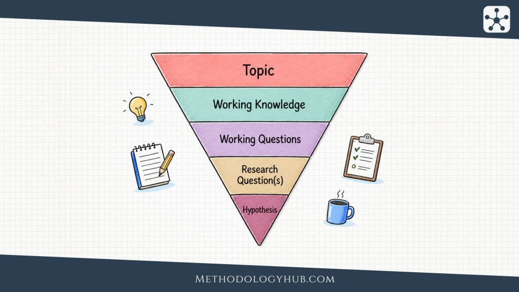
A good regression question is usually more specific than “are these variables related?” It asks something like: how much higher is the expected outcome when the predictor increases by one unit? Does the relationship remain after adjusting for other variables? How much uncertainty is attached to the estimate? Does the model fit the data reasonably well? Are there patterns in the residuals that suggest the model is wrong?
When regression analysis is used
Regression analysis is used when the research question involves a measurable outcome and one or more possible predictors. The outcome may be continuous, binary, counted, ordered, or measured over time. The type of outcome matters because it determines which kind of regression model is appropriate.
Regression is common when researchers want to estimate an association while accounting for other variables. For example, a study may examine whether physical activity is associated with blood pressure while adjusting for age and baseline body mass index. A school study may examine whether attendance predicts exam performance while accounting for prior achievement. A laboratory study may examine whether concentration predicts reaction rate while controlling for temperature.
Typical uses of regression analysis
- Estimating effects: measuring how much the outcome changes when a predictor changes.
- Making predictions: estimating likely outcomes for new observations.
- Adjusting for covariates: estimating a relationship while accounting for other variables.
- Testing hypotheses: checking whether a coefficient differs from zero under model assumptions.
- Comparing predictors: studying which variables are associated with the outcome in the same model.
- Checking theoretical relationships: examining whether data are consistent with an expected pattern.
Regression is especially useful when the question requires more than a simple comparison. If you only want to compare two group averages, a group comparison may be enough. If you want to compare those groups while adjusting for baseline differences or including several predictors at once, regression becomes more useful.
Where regression fits in a research workflow
Regression usually comes after basic data checking and descriptive analysis. First, you define the outcome and predictors. Then you inspect distributions, missing data, measurement scales, and possible outliers. A scatter plot or grouped summary can show whether the relationship looks roughly linear or whether another model form may be needed. Only then does it make sense to estimate the regression model.
After the model is estimated, the work is not finished. Regression output needs interpretation and checking. The coefficient table tells part of the story, but residual plots, influence checks, confidence intervals, and model fit measures are also important. A model can produce a clean table and still be a poor description of the data.
Regression analysis terms explained
Regression analysis becomes easier once the main terms are clear. Many errors in interpretation happen because people read the output without understanding what the rows and columns refer to. The terms below appear in almost every regression discussion.
Dependent variable and independent variable
The dependent variable is the outcome the model tries to explain or predict. It is often written as Y. The independent variable is a predictor used to explain or predict the outcome. It is often written as X. These names can be misleading because a predictor is not always truly independent in a causal sense. In regression output, “independent variable” usually means “variable placed on the predictor side of the model.”
For example, in a study of exam performance, the exam score may be Y and study hours may be X. In a clinical study, blood pressure after treatment may be Y, while treatment group, age, and baseline blood pressure may be predictors. In an environmental study, lung function may be Y, while pollution exposure, age, and smoking status may be predictors.
Coefficient and intercept
A regression coefficient estimates how much the outcome changes when a predictor increases by one unit, while other variables in the model are held constant. If the coefficient is positive, higher predictor values are associated with higher outcome values. If it is negative, higher predictor values are associated with lower outcome values.
The intercept is the expected value of Y when all predictors equal zero. Sometimes this has a meaningful interpretation. Sometimes it is only a mathematical anchor. If zero is outside the observed or meaningful range of the predictor, the intercept should not be overinterpreted.
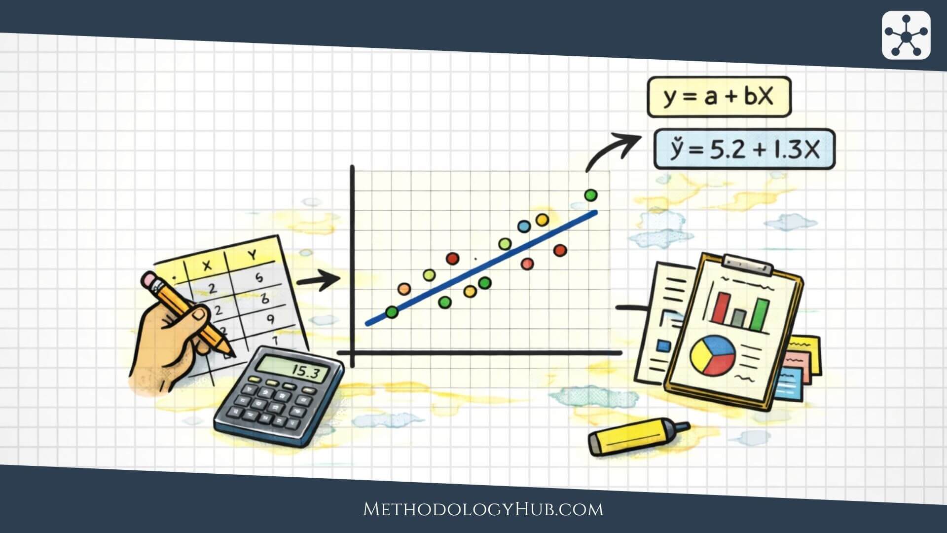
Fitted value and residual
A fitted value, often written as ŷ, is the model’s predicted value for an observation. A residual is the difference between the observed value and the fitted value. In simple terms, the residual is the model’s error for that observation.
Residuals are important because they show what the model misses. If residuals look random, the model may be a reasonable summary. If residuals show a curve, a funnel shape, clusters, or time patterns, the model may be missing something important.
Coefficient table and model fit
The coefficient table usually contains the intercept, each predictor, the estimated coefficient, the standard error, a test statistic, a p-value, and often a confidence interval. This table is where individual predictors are interpreted. It tells you the estimated effect, how uncertain that estimate is, and whether the data give evidence that the coefficient differs from zero under the model.
Model fit statistics give a different kind of information. R-squared, adjusted R-squared, residual standard error, RMSE, AIC, BIC, or other measures may be reported depending on the model. These measures do not replace coefficient interpretation. They help evaluate how well the model describes or predicts the outcome.
Regression equation and formulas
The regression equation is the part of the model that turns predictors into fitted values. It is useful because it makes the model explicit. Instead of saying vaguely that X is related to Y, the equation says how Y is estimated from X.
Simple linear regression equation
Simple linear regression uses one predictor to estimate one numerical outcome. The model fits a straight line through the data. The line has an intercept and a slope. The intercept places the line in the data space. The slope gives the expected change in Y for a one-unit increase in X.
If b is 2.5, the model estimates that Y increases by 2.5 units for each one-unit increase in X. If b is -2.5, the model estimates that Y decreases by 2.5 units for each one-unit increase in X. The coefficient is therefore an effect-size estimate in the units of the outcome.
Slope and intercept formulas
In simple linear regression, the slope can be written as the covariance between X and Y divided by the variance of X. This shows why the slope depends on how X and Y move together and on how much X varies.
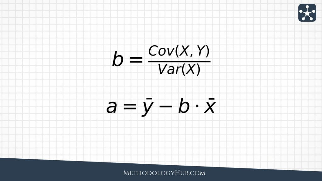
This formula also helps explain the connection between regression and correlation. Correlation is standardized, so it has no units. The slope is not standardized. It is expressed in Y-units per X-unit. That makes regression especially useful when you want an interpretable effect size.
Multiple regression equation
Multiple regression includes more than one predictor. The equation estimates Y from several X variables at the same time. Each coefficient is interpreted while holding the other predictors in the model constant.
The phrase “holding other predictors constant” is central. Suppose a model estimates reading score using study time, prior score, and attendance. The coefficient for study time is not simply the raw relationship between study time and reading score. It is the estimated relationship after accounting for prior score and attendance in the same model.
Least squares method
Linear regression usually uses the least squares method. The model chooses the intercept and coefficients so that the squared residuals are as small as possible overall. Squaring the residuals makes large errors count more heavily and prevents positive and negative errors from canceling each other out.
Types of regression analysis
Different regression models are used for different outcome variables and study designs. The most important first question is not which model sounds advanced. The most important question is what kind of outcome you have.
Simple linear regression
Simple linear regression uses one predictor to model a continuous outcome. It is useful when the relationship can be summarized with a straight line and the goal is to estimate a slope. For example, a researcher may model reaction time using age, or plant height using nutrient concentration in a controlled experiment.
Simple linear regression is easy to visualize because the fitted model is a line on a scatter plot. This makes it a good starting point for understanding regression. It also makes assumption problems easier to see. If the scatter plot is strongly curved, the straight-line model may not be appropriate.
Multiple linear regression
Multiple linear regression uses several predictors to model a continuous outcome. It is useful when the outcome has several plausible explanations or when the researcher needs to adjust for covariates. For example, a study of blood pressure may include age, body mass index, baseline blood pressure, and treatment group in the same model.
Multiple regression can be more informative than a series of simple regressions because predictors often overlap. A variable may look important by itself but become less important after adjusting for another variable. That change is not a failure of regression. It is often the reason regression is being used.
Logistic regression
Logistic regression is used when the outcome is binary, such as disease present or absent, pass or fail, complication or no complication, event or no event. Instead of predicting an ordinary numerical value, logistic regression models the probability of the event.
The coefficients in logistic regression are often interpreted through odds ratios. This makes interpretation less direct than in linear regression, but the basic idea is similar: the model estimates how the outcome probability changes with predictors. Logistic regression is common in medicine, epidemiology, psychology, education, and social research.
Other regression models
Many other regression models exist because not every outcome behaves like a continuous or binary variable. Count outcomes may need Poisson or negative binomial regression. Ordered outcome categories may need ordinal regression. Repeated measurements may need mixed models or generalized estimating equations. Time-to-event outcomes may need survival models.
You do not need to memorize every regression family to understand the principle. The outcome and data structure determine the model. A count, a probability, an ordered category, and a repeated measurement are different kinds of information. A good regression model respects those differences.
How to interpret regression results
Interpreting regression results means reading the output as a connected set of evidence. The coefficient estimates the relationship. The standard error and confidence interval show uncertainty. The p-value tests a narrow statistical claim. R-squared and RMSE describe model fit or prediction error. Residuals show where the model misses.
Regression coefficients
The coefficient is usually the first number people read. In linear regression, it tells you the expected change in Y for a one-unit increase in X, holding the other predictors constant. The unit matters. If X is measured in years, the coefficient is change in Y per year. If X is measured in milligrams, the coefficient is change in Y per milligram. If X is coded as a group indicator, the coefficient is the expected difference between the coded group and the reference group.
A coefficient should be interpreted with the outcome unit, predictor unit, and model context. A coefficient of 3 means very different things if the outcome is test points, blood pressure, reaction time, or pollutant concentration. The number does not interpret itself.
Standard errors, p-values, and confidence intervals
A standard error describes the uncertainty in a coefficient estimate. A smaller standard error relative to the coefficient means the estimate is more precise. A larger standard error means the estimate is more uncertain.
A p-value usually tests whether the coefficient differs from zero under the model assumptions. It does not tell you whether the effect is important, causal, or useful. A tiny coefficient can become statistically significant in a large sample. A meaningful coefficient can fail to reach statistical significance in a small or noisy sample.
A confidence interval is often more useful than the p-value because it shows a range of plausible coefficient values. If the interval is narrow, the estimate is relatively precise. If it is wide, the data do not pin down the effect very well.
R-squared and adjusted R-squared
R-squared describes the proportion of variation in the outcome that is explained by the model, compared with a model that uses only the outcome mean. An R-squared of 0.60 means that the model explains about 60% of the observed variation in Y in that dataset.
R-squared can be useful, but it is easy to overread. A high R-squared does not prove causation. A low R-squared does not always mean the model is useless. In some fields, outcomes are naturally noisy, and a modest R-squared may still be scientifically useful. In prediction tasks, an error measure may be more informative than R-squared alone.
Adjusted R-squared penalizes model complexity. It is useful when comparing models with different numbers of predictors. Adding more predictors can increase ordinary R-squared even if those predictors add little real value. Adjusted R-squared is more cautious.
RMSE and prediction error
RMSE, or root mean squared error, describes the typical size of prediction errors in the units of the outcome. If the outcome is measured in test points, RMSE is in test points. If the outcome is measured in millimeters of mercury, RMSE is in millimeters of mercury. This makes it easier to judge whether prediction error is large or small in context.
Regression assumptions and diagnostics
Regression models rely on assumptions. These assumptions are not decorations. They affect whether coefficient estimates, standard errors, p-values, confidence intervals, and predictions can be trusted. Assumptions are checked through plots, diagnostics, and judgment about the study design.
Linearity
In linear regression, the relationship between predictors and the outcome should be reasonably described by a linear form. This does not mean the real world must be perfectly straight. It means the straight-line model should be an acceptable summary for the question being asked.
A scatter plot can show whether a simple linear relationship is reasonable. Residual plots can show whether the model is missing a curve. If residuals form a clear pattern, the model may need transformation, nonlinear terms, interactions, or a different model.
Independence
Many regression models assume observations are independent. If the same person is measured repeatedly, if students are nested within classrooms, or if samples are clustered within laboratories, independence may be violated. Treating dependent observations as independent can make results look more precise than they are.
When dependence is part of the data structure, the model should account for it. Options may include mixed models, clustered standard errors, repeated-measures models, longitudinal models, or other approaches depending on the design.
Constant variance
Constant variance means the spread of residuals is roughly similar across fitted values. If residuals form a funnel shape, the model may have heteroscedasticity. This can affect standard errors, tests, and intervals. It may also signal that the model fits some parts of the data better than others.
Normality of residuals
For ordinary linear regression, normality of residuals is mainly important for inference, especially in small samples. The residuals do not need to be perfectly normal, but severe departures can affect p-values and confidence intervals. Large samples are often more forgiving, but diagnostic checking is still useful.
Outliers and influential observations
Outliers are unusual observations. Influential observations are points that strongly affect the fitted model. A point can be influential because it has an unusual predictor value, an unusual outcome value, or both. Influential points are not automatically wrong, but they need attention.
The question is not simply whether to delete a point. First, check whether the value is a measurement error, data entry error, or valid observation. Then examine how much the model changes with and without it. If conclusions depend on one point, the report should make that sensitivity clear.
Multicollinearity
Multicollinearity happens when predictors in a multiple regression model are strongly related to each other. The model may still predict well, but individual coefficients can become unstable and hard to interpret. Standard errors may become large. Coefficients may change signs when predictors are added or removed.
Multicollinearity is common when several variables measure similar constructs. For example, several cognitive test scores may overlap. Several measures of body size may overlap. Several environmental exposures may rise and fall together. The response may be to combine variables, choose one representative measure, use dimension reduction, or interpret the model more cautiously.
Regression analysis step by step
A regression analysis should be done as a sequence of decisions, not as one software command. The steps below apply to many regression settings, even though the details change with the model type.
Step 1 – define the outcome and predictors
Start by defining the outcome variable clearly. What exactly is Y? What unit is it measured in? What time point does it refer to? Then define the predictors. Which variables are being used to explain or predict Y? Are they measured before the outcome? Are they continuous, categorical, binary, ordered, or time-based?
Step 2 – inspect the data
Before fitting a model, inspect the data. Check distributions, missing values, impossible values, duplicated records, outliers, and measurement scales. Plot the outcome against key predictors. A regression model can calculate with poor data, but it cannot make poor data reliable.
Step 3 – choose the model type
Choose the model based on the outcome and design. A continuous outcome may use linear regression. A binary outcome may use logistic regression. Counts may need count regression. Repeated measurements may need a model that handles dependence. The model should match the data structure.
Step 4 – fit the model
Estimate the model and record the main outputs. These usually include coefficients, standard errors, confidence intervals, p-values, fitted values, residuals, and fit measures. Do not interpret the p-values before checking whether the model makes sense.
Step 5 – check diagnostics
Look at residual plots, outliers, influential observations, and assumption checks. In multiple regression, check whether predictors overlap too strongly. In prediction work, check performance on data not used to fit the model if possible.
Step 6 – interpret the results
Interpret the coefficients in plain language. State the outcome unit, predictor unit, direction, size, uncertainty, and limitations. Avoid saying “X causes Y” unless the study design supports a causal claim. Most regression models describe conditional associations, not automatic causes.
Regression analysis examples
Examples help show what regression can and cannot do. In each example, the model estimates a relationship between an outcome and predictors. The interpretation still depends on the design, measurement quality, assumptions, and possible missing variables.
Example 1 – study time and exam score
An education researcher may model exam score using study time. The outcome is exam score. The predictor is study time. A positive coefficient would mean that students with more study time tend to have higher scores, on average.
The coefficient might be interpreted as the expected change in exam score for each additional hour of study. But the result does not automatically prove that study time caused the score increase. Prior knowledge, attendance, sleep, access to support, and study quality may also matter. Regression can describe the association and adjust for measured covariates, but unmeasured factors may still remain.
Example 2 – blood pressure after treatment
A clinical researcher may model blood pressure after treatment using treatment group, baseline blood pressure, age, and body mass index. Here regression helps compare treatment groups while accounting for differences that existed before treatment.
This example shows why multiple regression is useful. If one treatment group happened to have higher baseline blood pressure, a simple comparison of final blood pressure might be misleading. Including baseline blood pressure in the model can make the comparison more informative. The model still depends on study design and assumptions, but it can give a clearer adjusted estimate.
Example 3 – plant growth and nutrient concentration
In an experimental biology setting, a researcher may model plant height using nutrient concentration. If the relationship is roughly linear across the studied range, simple linear regression may estimate how much plant height changes per unit increase in nutrient concentration.
If the relationship rises at first and then levels off, a simple straight-line model may be too crude. A nonlinear term or different model may be needed. This example shows why the scatter plot and residuals matter before interpreting the coefficient as if it describes the whole relationship.
Example 4 – disease status and exposure
An epidemiological study may use logistic regression when the outcome is disease status. The predictors may include exposure level, age, sex, and other covariates. The model estimates how the probability or odds of disease differ with exposure and covariates.
The interpretation needs care because logistic regression coefficients are not ordinary changes in the outcome. They are often converted into odds ratios. The result can be useful for studying risk factors, but causal interpretation still depends on the design and control of confounding.
Common mistakes in regression analysis
Regression analysis is powerful, but that power makes mistakes easier to hide. A table of coefficients can look official even when the model is poorly chosen, the data are weak, or the interpretation goes beyond the design.
Treating regression as causation
A regression coefficient is not automatically a causal effect. It is an estimated association conditional on the variables in the model. Causal interpretation requires stronger design, careful timing, control of confounding, and a defensible argument about what would have happened otherwise.
Leaving out important variables
Omitted variable bias can occur when an important variable is left out of the model and is related to both the predictor and the outcome. The included predictor may then appear to have an effect that partly belongs to the missing variable.
Ignoring nonlinearity
A straight-line model can be misleading when the relationship is curved. The model may average over a pattern that changes across the range of X. Residual plots and scatter plots are the easiest early checks.
Overfitting the data
Overfitting happens when a model learns the noise in the sample rather than a pattern that generalizes. This is common when many predictors are used with limited data. The model may fit the current dataset well but perform poorly on new data.
Ignoring multicollinearity
When predictors strongly overlap, individual coefficients can become unstable. The model may still have good overall fit, but it becomes hard to say which predictor is responsible for which part of the association.
Reporting output without interpretation
Regression output is not self-explanatory. A good report explains what the coefficient means in the units of the study, how uncertain it is, whether the model is appropriate, and what limitations remain.
Conclusion
Regression analysis is useful because many research questions involve outcomes that change with other variables. A regression model gives more than a yes-or-no answer. It estimates a relationship, gives an equation, produces fitted values, shows residuals, and attaches uncertainty to the coefficients.
The strength of regression is also the reason it needs care. A model can include several predictors, adjust for covariates, and produce polished tables. But the model still depends on the quality of the data, the choice of outcome, the measurement of predictors, the assumptions, and the study design. Regression can describe, estimate, and predict. It does not automatically explain cause and effect.
The safest way to use regression is to start with the question, choose the model based on the outcome and design, inspect the data, check the diagnostics, and interpret the coefficients in plain language. A good regression analysis is not just a fitted equation. It is a careful argument about what the data can and cannot support.
FAQs on Regression Analysis
What is regression analysis?
Regression analysis is a statistical method used to model how an outcome variable changes with one or more predictor variables.
What is regression analysis used for?
Regression analysis is used to estimate relationships, adjust for covariates, test hypotheses, make predictions, and quantify uncertainty around effects.
What is the difference between correlation and regression?
Correlation summarizes the direction and strength of association between two variables. Regression estimates an equation and shows how an outcome changes with one or more predictors.
What does a regression coefficient mean?
A regression coefficient estimates how much the outcome changes when a predictor increases by one unit, holding other variables in the model constant.
What does R-squared mean in regression analysis?
R-squared shows the proportion of variation in the outcome that is explained by the regression model in the observed data.
Can regression analysis prove causation?
Regression analysis does not automatically prove causation. Causal claims need a suitable study design, clear timing, control of confounding, and defensible assumptions.