Spearman’s rank correlation is a measure used in statistical analysis to describe the direction and strength of association between two variables after their values have been converted into ranks. It is often written as Spearman’s ρ, Spearman’s rho, or rs, and it is especially useful when the relationship is monotonic rather than strictly linear.
In many studies, the original values are less important than their order. A researcher may want to know whether students who rank higher in reading confidence also rank higher in reading comprehension, whether judges give similar rankings to a set of performances, or whether two ordinal rating scales move in the same direction. In such cases, Spearman’s correlation gives a compact way to describe how closely the two rankings agree.
This article explains what Spearman’s rank correlation is, how it differs from Pearson’s correlation, when to use it, how the formula works, how to calculate it by hand, how to interpret the result, and how to report Spearman’s correlation in academic writing.
What Is Spearman’s Rank Correlation?
Spearman’s rank correlation is a measure of association between two variables based on the ranks of their values. Instead of asking whether the raw values follow a straight-line pattern, it asks whether the order of the observations is similar across the two variables.
Imagine a teacher records two things for the same group of students: a classroom participation rating and a project score. The exact distance between ratings may not be easy to treat as equal. Still, the order may be meaningful. A student can be ranked first, second, third, and so on for participation, and the same students can be ranked again for the project score. Spearman’s rank correlation then examines whether students with higher participation ranks also tend to have higher project-score ranks.
Spearman’s rank correlation definition
Spearman’s rank correlation is a statistic that measures the direction and strength of a monotonic association between two variables by using ranks. Its value ranges from -1 to +1. A value near +1 means that higher ranks on one variable tend to go with higher ranks on the other. A value near -1 means that higher ranks on one variable tend to go with lower ranks on the other. A value near 0 means that the ranks do not show a clear increasing or decreasing pattern.
The word monotonic is important. A monotonic relationship moves mainly in one direction. As one variable increases, the other generally increases, or it generally decreases. The pattern does not need to form a perfect straight line. This is the main reason Spearman’s correlation can be useful when Pearson’s correlation feels too narrow for the shape of the data.
What Spearman’s correlation tells the reader
Spearman’s correlation tells the reader how similar two ordered patterns are. The sign gives the direction. A positive coefficient shows that the two sets of ranks tend to rise together. A negative coefficient shows that one set of ranks tends to rise while the other falls.
The size of the coefficient shows how closely the ranks follow that direction. A value of 0.80 and a value of -0.80 are equally strong in size, but they point in opposite directions. The first describes similar ordering. The second describes reversed ordering.
Ranks instead of raw values
The defining feature of Spearman’s rank correlation is that it works with order. The smallest value receives the lowest rank, the next smallest receives the next rank, and the process continues until all observations are ranked. Once the ranks have been assigned, the calculation examines the relationship between those ranks.
This makes the coefficient useful for ordinal data, such as satisfaction ratings, preference rankings, survey scales, classroom ratings, symptom severity categories, and other ordered measurements. It can also be used with quantitative variables when the raw values are skewed, contain unusual observations, or follow a curved but still steadily increasing or decreasing pattern.
Sample correlation and population correlation
In a research report, Spearman’s correlation is usually calculated from a sample. The sample value estimates the population association, but it does not give perfect knowledge of it. Two different samples from the same population may produce slightly different coefficients.
This distinction connects Spearman’s rank correlation with inferential statistics. A researcher may use the sample coefficient descriptively, simply to summarise the data in front of them. The analysis becomes inferential when the researcher tests whether the population correlation differs from zero or reports a confidence interval for the population value.
Key Assumptions of Spearman’s Rank Correlation
Spearman’s rank correlation is often introduced as a flexible alternative to Pearson’s correlation. That flexibility is real, but it does not mean the method has no conditions. The coefficient still needs paired observations, meaningful order, a suitable association pattern, and a study design that supports the interpretation being made.
Paired observations
Spearman’s correlation requires paired observations. Each case must have a value on both variables. If a student has a rank for reading confidence but no comprehension score, that pair cannot be used in the ordinary calculation unless missing data are handled through a planned method.
The pairing is what allows the ranks to be compared row by row. Spearman’s correlation is not comparing two unrelated lists. It is comparing two measurements taken from the same people, texts, schools, patients, plants, records, or other units of analysis.
Ordinal or quantitative variables
At minimum, both variables should have an order that makes sense. This can be natural order, such as low, medium, and high; ranked order, such as first through tenth; or numerical order, such as test scores or response times. The coefficient does not require equal distances between values in the same way Pearson’s correlation does.
Spearman’s rank correlation is not suitable for purely nominal categories, such as subject area, eye colour, or school type, unless those categories have been transformed into a meaningful ordered variable. A category code such as 1, 2, and 3 is not enough by itself. The order has to represent something real in the research data.
A monotonic relationship
The main pattern to check is monotonicity. A monotonic pattern means that as one variable increases, the other tends to increase, or as one variable increases, the other tends to decrease. The pattern may curve, flatten, or rise unevenly, but it should not repeatedly change direction.
A scatterplot can still be useful before calculating Spearman’s correlation. If the plot shows a general upward or downward movement, Spearman’s rho may give a fair summary. If the plot rises, falls, and rises again, a single rank correlation can hide the shape rather than explain it.
Independence of observations
Each pair of observations should be independent unless the analysis is designed for repeated or clustered data. If the same student appears several times, if many students come from the same classroom, or if several measurements come from the same patient, the ordinary coefficient may treat related observations as if they were separate.
This affects inference in particular. A coefficient can always be calculated, but a p-value based on independent pairs may be misleading when the design contains repeated measurements or nested groups. In such cases, the researcher may need a method that respects the structure of the data.
Ties in the ranks
Ties occur when two or more observations have the same value. They are common in rating scales. If several students receive the same score, or several respondents choose the same agreement category, those observations share rank positions.
The usual solution is to assign average ranks. If two observations would have occupied ranks 3 and 4, both receive rank 3.5. Statistical software usually handles ties automatically. When calculating by hand, ties deserve careful attention because the simple no-tie formula is exact only when all ranks are distinct.
Outliers and unusual observations
Spearman’s correlation is usually less sensitive to extreme raw values than Pearson’s correlation because it works with ranks. A very large value may only become the highest rank rather than pulling the calculation strongly through its original size.
This does not mean unusual observations can be ignored. A single observation with a very unexpected rank pattern can still affect the result, especially in a small sample. The researcher should check whether unusual points are data errors, special cases, or meaningful observations that belong in the analysis.
When to Use Spearman’s Correlation
Spearman’s correlation is appropriate when the research question asks whether two ordered variables tend to move together. It is often chosen when the original measurements are ordinal, when the relationship is monotonic but not clearly linear, or when raw values contain outliers that would make Pearson’s correlation difficult to interpret.
The method fits many academic situations. An education researcher may compare teacher rankings and student self-ratings. A psychology researcher may examine two ordered questionnaire scales. A health researcher may study whether symptom severity categories rise with another ordered clinical measure. In each case, the analysis is about ordered association rather than exact differences between raw values.
Use Spearman’s correlation for ordinal variables
Ordinal variables give information about order, but not necessarily about equal distances. A response scale from 1 to 5 may tell us that 5 is higher than 4 and 4 is higher than 3. It does not guarantee that the distance between 1 and 2 is the same as the distance between 4 and 5.
Spearman’s rank correlation is often a natural choice for this kind of data because it does not rely on those distances in the same way Pearson’s correlation does. The ranks carry the analysis. The coefficient asks whether higher positions on one variable tend to go with higher or lower positions on the other.
Use Spearman’s correlation for monotonic patterns
Some relationships are clearly increasing or decreasing but not linear. For example, a learning score may improve quickly at first as practice time increases, then improve more slowly after students have already practised a great deal. Pearson’s correlation may understate or distort that kind of curved association if the straight-line summary is not suitable.
Spearman’s correlation can describe the ordered movement more comfortably because it focuses on rank order. If students with more practice generally receive higher scores, even along a curve, the rank-based coefficient may still be high.
Use Spearman’s correlation when outliers affect raw values
Outliers can have a strong effect on Pearson’s correlation because Pearson’s coefficient uses the original numerical values. Spearman’s correlation reduces that influence by replacing values with ranks. An extremely high score becomes the highest rank, but its exact distance from the next score is not used in the same way.
This can be helpful when unusual raw values are real and should remain in the dataset. It does not remove the need to inspect the data. It simply gives a rank-based summary that may better match the research question.
Use Spearman’s correlation for association, not cause
Spearman’s rank correlation describes association. It does not show that one variable caused another. A positive Spearman’s correlation between class participation and final grade may fit the idea that participation supports learning, but it may also reflect confidence, prior knowledge, teacher expectations, access to resources, or other variables not included in the analysis.
Causal claims need support from the study design, not only from the coefficient. Experiments, longitudinal evidence, theoretical reasoning, measurement quality, and control variables all shape how far an interpretation can go.
Formula for Spearman’s Rank Correlation
The formula for Spearman’s rank correlation is easiest to understand after remembering what the statistic does. It compares two rankings for the same observations. When the ranks are similar, the coefficient is positive. When the ranks are reversed, the coefficient is negative. When rank differences are mixed and irregular, the coefficient moves closer to zero.
![]()
In this formula, d is the difference between the two ranks for each observation, d2 is that difference squared, Σd2 is the sum of all squared rank differences, and n is the number of paired observations.
Formula in words
The no-tie formula says that Spearman’s correlation becomes smaller as the rank differences become larger. If every observation has the same rank on both variables, every rank difference is zero. The sum of squared differences is zero, so the coefficient becomes +1.
If the rankings are perfectly reversed, the rank differences are as large as they can be. The coefficient becomes -1. Most real datasets fall between those two extremes. Some pairs have similar ranks, some have different ranks, and the final value summarises the overall pattern.
Spearman’s correlation as Pearson’s correlation of ranks
There is another way to understand the same statistic. Spearman’s correlation can be calculated by first ranking both variables and then applying the Pearson correlation formula to those ranks. This view is useful because it also explains what to do when there are ties.
When there are no ties, the short formula using squared rank differences gives the same result. When ties are present, the safer approach is to assign average ranks and calculate Pearson’s correlation on those rank values. Statistical software usually does this automatically.
What the formula is doing
The formula begins with the rank difference for each observation. If a student is ranked 2nd on one variable and 3rd on another, the difference is -1 or +1, depending on which rank is subtracted from which. Squaring the difference makes the sign irrelevant. A difference of -1 and a difference of +1 both become 1.
The calculation then adds all squared rank differences. A small total means that the two rankings are similar. A large total means that many observations have very different positions in the two rankings. The final part of the formula standardises the result so it falls between -1 and +1.
How ties change the calculation
Ties are common in practical data. Several respondents may choose the same rating, or several students may receive the same score. When ties occur, each tied value receives the average of the rank positions it occupies.
For example, if two observations share the second and third positions, both receive rank 2.5. If three observations share ranks 4, 5, and 6, all three receive rank 5. The coefficient can then be calculated from the ranked variables. In many software packages, selecting Spearman’s correlation is enough; the tie handling happens behind the scenes.
Calculating Spearman’s Rank Correlation
Spearman’s rank correlation is usually calculated with statistical software, but a hand calculation is useful because it shows what the coefficient is doing. The example below uses a small dataset with no tied values so that the simple formula can be shown clearly.
Suppose a teacher records a practice score and a final project score for six students. The question is whether students with higher practice scores also tend to receive higher final project scores.
| Student | Practice score | Final project score |
|---|---|---|
| A | 58 | 61 |
| B | 62 | 66 |
| C | 65 | 64 |
| D | 72 | 75 |
| E | 78 | 82 |
| F | 84 | 79 |
Step 1: Rank each variable
The smallest practice score receives rank 1, and the largest receives rank 6. The same ranking process is then applied to the final project scores. Because this example has no tied values, every rank is a whole number.
| Student | Practice score | Practice rank | Final score | Final rank |
|---|---|---|---|---|
| A | 58 | 1 | 61 | 1 |
| B | 62 | 2 | 66 | 3 |
| C | 65 | 3 | 64 | 2 |
| D | 72 | 4 | 75 | 4 |
| E | 78 | 5 | 82 | 6 |
| F | 84 | 6 | 79 | 5 |
Step 2: Find the rank differences
Next, subtract one rank from the other for each student. The direction of subtraction does not affect the final no-tie formula because the differences will be squared.
| Student | Practice rank | Final rank | d | d2 |
|---|---|---|---|---|
| A | 1 | 1 | 0 | 0 |
| B | 2 | 3 | -1 | 1 |
| C | 3 | 2 | 1 | 1 |
| D | 4 | 4 | 0 | 0 |
| E | 5 | 6 | -1 | 1 |
| F | 6 | 5 | 1 | 1 |
Sum of squared rank differences:
Σd2 = 0 + 1 + 1 + 0 + 1 + 1 = 4
Step 3: Insert the values into the formula
The sample size is 6, and the sum of squared rank differences is 4. These values can now be placed into the formula.
Calculation:
ρ = 1 – [6(4) / 6(62 – 1)]
ρ = 1 – [24 / 6(35)]
ρ = 1 – [24 / 210]
ρ = 0.886
The result is approximately 0.89. In this small example, practice score and final project score have a strong positive rank association. Students with higher practice-score ranks generally also have higher final-project ranks, although the two rankings are not perfectly identical.
What the result says in the example
The result does not say that practice caused the final project score. It also does not say that every additional practice point creates a fixed increase in the project score. It says that, in this dataset, students who ranked higher on practice tended to rank higher on the final project.
This is the kind of statement Spearman’s rank correlation supports well. It keeps the focus on ordered association, which is exactly what the coefficient was designed to summarise.
Handling Tied Ranks in Spearman’s Correlation
Tied ranks deserve their own attention because they appear often in real research data. The hand calculation above used scores with no repeated values, which made the short formula easy to use. Many actual datasets are less tidy. Rating scales, rubric scores, category scales, and rounded measurements often contain repeated values, and those repeated values affect how ranks are assigned.
The presence of ties does not mean Spearman’s rank correlation has to be abandoned. It means the ranking step needs to be handled carefully. Once tied values receive average ranks, the coefficient can be calculated from those ranks, usually through software. The important point is to know what the software is doing and to report the analysis in a way that fits the data.
Why ties occur
Ties occur when two or more observations have the same value on a variable. In a five-point satisfaction scale, many respondents may choose the same category. In a classroom rubric, several students may receive the same score. In a clinical severity scale, many patients may fall into the same ordered group.
This is not a defect in the data. It often reflects the way the variable was measured. A scale with only five response options cannot create a unique rank for every participant in a large sample. The analysis should therefore respect the measurement level rather than pretend that every case has a unique position.
Average ranks for tied values
The standard approach is to give tied values the average of the ranks they would have occupied. Suppose four students receive the following rubric scores: 70, 80, 80, and 90. The score of 70 receives rank 1. The two scores of 80 would occupy ranks 2 and 3, so each receives rank 2.5. The score of 90 receives rank 4.
The same rule applies to larger groups of tied values. If three observations share ranks 5, 6, and 7, each receives rank 6. This keeps the total amount of rank information in the dataset in balance. It also avoids making an arbitrary choice about which tied observation should be placed above another.
Example of tied ranks
Consider a short example with six students rated on classroom engagement from 1 to 5. If the engagement ratings are 2, 3, 3, 4, 5, and 5, the two students with rating 3 share ranks 2 and 3, so each receives 2.5. The two students with rating 5 share ranks 5 and 6, so each receives 5.5.
| Student | Engagement rating | Rank used in analysis |
|---|---|---|
| A | 2 | 1 |
| B | 3 | 2.5 |
| C | 3 | 2.5 |
| D | 4 | 4 |
| E | 5 | 5.5 |
| F | 5 | 5.5 |
If another variable is also ranked, Spearman’s correlation can then compare the two sets of rank values. Because the ranks now include decimals, it is usually easier to use software or the Pearson-on-ranks approach rather than the simple squared-difference formula shown earlier.
What software usually does
Most statistical software handles tied ranks by assigning average ranks and then calculating the correlation from the ranked variables. The exact p-value method may vary, especially with small samples or many ties. For large samples, many programs use an approximation. For small samples, exact or permutation-based methods may be available.
This is one reason the methods section of a research report should be clear. If the dataset contains many ties, especially because both variables are short ordinal scales, it can be helpful to state that Spearman’s rank correlation was calculated using average ranks for tied values. The reader then understands how repeated values were handled.
When ties are frequent
Frequent ties reduce the amount of ordering information in the data. A five-point scale used with 500 respondents may still be useful, but it cannot distinguish 500 unique ranks. The coefficient can be calculated, yet the interpretation should remember that the scale is coarse.
In some studies, a large number of ties may suggest that a different method should also be considered. For example, if both variables have only two or three ordered categories, a table-based analysis or an ordinal model may sometimes give a fuller view. Spearman’s correlation can still provide a readable association measure, but it should fit the question rather than be chosen automatically.
Interpreting Spearman’s Correlation
Interpreting Spearman’s correlation means reading the coefficient together with the variables, the sample, the graph, and the research design. The number itself is useful, but it should not be treated as a complete interpretation on its own.
![]()
Positive Spearman’s correlation
A positive Spearman’s correlation means that higher ranks on one variable tend to go with higher ranks on the other. If motivation rating and homework completion have a positive Spearman’s correlation, students with higher motivation ranks generally also have higher homework-completion ranks.
The word generally leaves room for real data. A positive coefficient does not require every case to fit the pattern. It says that the overall ranking pattern moves upward.
Negative Spearman’s correlation
A negative Spearman’s correlation means that higher ranks on one variable tend to go with lower ranks on the other. For example, if rank in waiting time is negatively associated with rank in satisfaction, people with longer waiting times may tend to give lower satisfaction ratings.
The sign does not make the result stronger or weaker by itself. A value of -0.70 is stronger than a value of +0.25 because -0.70 is farther from zero. The negative sign only tells the direction.
Spearman’s correlation near zero
A value near zero means that the two sets of ranks do not show a clear monotonic pattern. Higher ranks on one variable are not consistently paired with higher or lower ranks on the other.
This should be read carefully. A near-zero coefficient does not prove that the variables have no relationship of any kind. The relationship might be nonmonotonic, the sample might be small, the measurements might be noisy, or the variables might be connected only within subgroups. A plot and study context help prevent overreading a single value.
Strength of the coefficient
Many textbooks offer rough labels such as weak, moderate, or strong. These labels can help beginners, but they should be used with care. A coefficient that looks small in one field may be meaningful in another field, especially when the variables are difficult to measure or the outcome is influenced by many conditions.
A useful interpretation names the variables and the direction of the pattern. Instead of writing only that there was a moderate positive correlation, a clearer sentence might say that students with higher self-rated reading confidence tended to have higher ranks in reading comprehension.
Statistical significance and uncertainty
A significance test for Spearman’s correlation usually evaluates whether the population rank correlation could be zero. A small p-value suggests that the sample result would be unusual under a zero-correlation assumption, given the method used.
The p-value should not replace the coefficient. A very small association can become statistically significant in a large sample, while a visibly large association may be uncertain in a small sample. When the coefficient is central to the study, reporting a confidence interval can help readers see the plausible range of the population association.
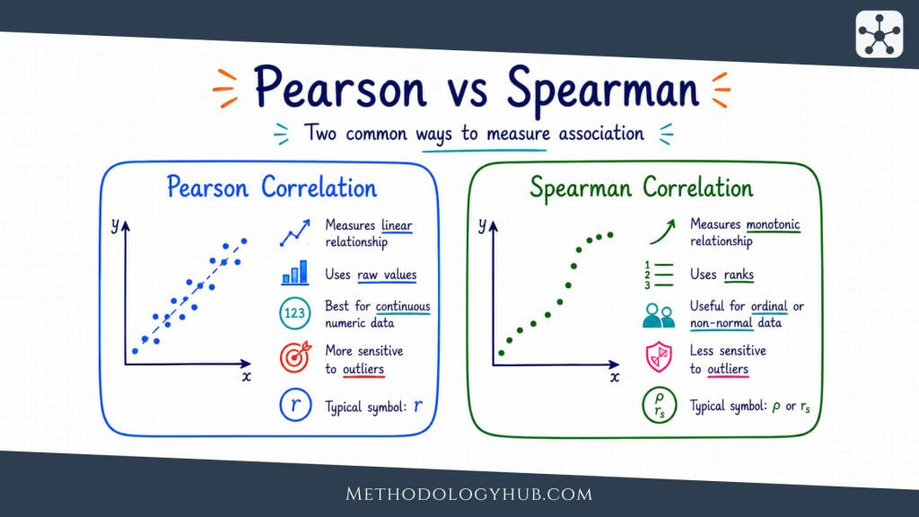
Spearman vs Pearson Correlation
Spearman’s rank correlation and Pearson’s correlation are both used to describe association between two variables, but they answer different questions. Pearson’s correlation uses the original numerical values and describes linear association. Spearman’s correlation uses ranks and describes monotonic association.
The difference becomes clear when the relationship is curved. If the points form a steady upward curve, Pearson’s correlation may not fully capture the pattern because it tries to summarise the data with a straight line. Spearman’s rank correlation may describe the same data more naturally because the order is still mostly increasing.
Measurement level
Pearson’s correlation is usually used with quantitative variables measured on interval or ratio scales. Spearman’s correlation can be used with ordinal variables because it only needs meaningful order. This is one reason Spearman’s correlation is common in research involving rating scales and ranked judgments.
For example, if two judges rank the same set of essays from strongest to weakest, Spearman’s correlation can measure how similarly the judges ordered the essays. Pearson’s correlation would not be the natural first choice unless the scores were numerical and the distances between values were meaningful.
Shape of the relationship
Pearson’s correlation fits straight-line patterns. Spearman’s rank correlation fits monotonic patterns. Every linear increasing relationship is monotonic, but not every monotonic relationship is linear.
This means that the two coefficients can sometimes lead to different impressions. If the data are roughly linear and measured quantitatively, Pearson’s correlation may be appropriate. If the data are ordered, skewed, or steadily curved, Spearman’s correlation may better match the question.
| Aspect | Spearman’s rank correlation | Pearson correlation |
|---|---|---|
| Main focus | Monotonic association between ranks | Linear association between raw values |
| Data type | Ordinal or quantitative | Usually quantitative |
| Outliers | Less affected by extreme raw values | Can be strongly affected by extreme values |
| Typical use | Rankings, rating scales, monotonic curved patterns | Continuous variables with a straight-line pattern |
Choosing between the two
The choice should follow the research question and the data. If the question is about a linear relationship between two quantitative variables, and the scatterplot supports a straight-line reading, Pearson’s correlation is often suitable. If the question is about ordered association, ordinal variables, or a monotonic pattern that is not straight, Spearman’s rank correlation may be the better fit.
It is sometimes useful to calculate both, especially during exploratory analysis, but the report should explain the coefficient that best matches the planned interpretation. The analysis should not switch between them only because one gives a stronger or more convenient result.
Reporting Spearman’s Rank Correlation
A clear report gives the coefficient, the sample size, the p-value when a test is used, and a sentence explaining the result in the language of the study. The report should also mention if ties were common, if the variables were ordinal, or if Spearman’s correlation was chosen because the relationship was monotonic rather than linear.
Basic reporting format
A short statistical report might look like this: “A Spearman’s rank correlation showed a positive association between reading-confidence rank and comprehension-score rank, ρ = .62, n = 48, p = .003.”
This sentence gives the method, direction, variables, coefficient, sample size, and p-value. A fuller version could add a confidence interval, a description of the scatterplot, or a reason for using a rank-based coefficient.
Reporting Spearman’s correlation with a confidence interval
When the result is central to the research question, a confidence interval gives useful information about precision. A report might state: “The association was positive, ρ = .46, 95% CI [.18, .67], suggesting that higher motivation ranks tended to occur with higher homework-completion ranks.”
The confidence interval helps the reader see whether the estimate is precise or uncertain. A wide interval does not make the result useless, but it does mean the population association is not estimated very tightly.
Reporting non-significant Spearman correlations
Non-significant results should be reported carefully. A result such as ρ = .14, p = .28 does not prove that there is no association. It means the sample did not provide enough evidence to reject a zero population association under the test used.
This distinction is especially important in small samples. A non-significant result may reflect limited power or noisy measurement rather than a clearly absent relationship. Reporting the coefficient and confidence interval helps keep that uncertainty visible.
Writing the interpretation
The interpretation should name the variables and describe the pattern. Instead of writing only that there was a strong Spearman’s correlation, explain what was ordered similarly or differently. A reader should know what the coefficient means in the study without having to translate it alone.
Association language is safest unless the study design supports a causal claim. Phrases such as “was associated with,” “tended to rank higher with,” or “showed a positive rank association with” keep the interpretation close to what Spearman’s correlation can show.
Conclusion
Spearman’s rank correlation gives researchers a practical way to describe association between two ordered variables. It is especially useful when the research question concerns rank order, ordinal scales, or a monotonic relationship that does not fit neatly into a straight-line pattern.
The coefficient is simple to read once its logic is clear. Positive values show that higher ranks on one variable tend to go with higher ranks on the other. Negative values show that higher ranks on one variable tend to go with lower ranks on the other. Values near zero show that there is no clear monotonic pattern in the analysed data.
A strong analysis does more than calculate the coefficient. It checks whether the observations are paired, whether the variables have meaningful order, whether the relationship is monotonic, and whether ties or unusual observations need attention. It also reports the result in a way that keeps uncertainty and study design visible.
FAQs on Spearman’s Rank Correlation
What is Spearman’s rank correlation?
Spearman’s rank correlation is a statistic that measures the direction and strength of a monotonic association between two variables after their values have been converted into ranks. It ranges from -1 to +1.
When should I use Spearman’s correlation?
Use Spearman’s correlation when both variables have a meaningful order and the research question concerns monotonic association. It is often used for ordinal variables, rankings, rating scales, skewed variables, or curved relationships that move mainly in one direction.
What does a Spearman’s correlation of 0 mean?
A Spearman’s correlation of 0 means that the ranks do not show a clear increasing or decreasing pattern in the analysed data. It does not prove that the variables are completely unrelated, because a different kind of relationship may still exist.
What is the difference between Spearman and Pearson correlation?
Spearman’s correlation uses ranks and measures monotonic association. Pearson correlation uses the original numerical values and measures linear association. Spearman’s correlation is often better for ordinal data, ranked data, or monotonic relationships that are not straight lines.
Can Spearman’s rank correlation show causation?
No. Spearman’s rank correlation describes association between two variables. It does not show that one variable caused the other to change. Causal claims require support from the study design and wider evidence.
How do you report Spearman’s rank correlation?
A report usually includes the coefficient, sample size, p-value if a test was used, and a plain interpretation. For example: A Spearman’s rank correlation showed a positive association between the two variables, ρ = .62, n = 48, p = .003.