Hypothesis testing is a statistical analysis procedure for using sample data to evaluate a claim about a population. A researcher rarely has access to every possible person, score, record, classroom, patient, or measurement. Instead, the researcher studies a sample and asks whether the observed result is strong enough to challenge a starting assumption.
This article explains what hypothesis testing is, how null and alternative hypotheses work, how p-values and significance levels are interpreted, which statistical tests are often used, and how to perform a hypothesis test by following a seven-step procedure.
What Is Hypothesis Testing?
Hypothesis testing is a method in inferential statistics that evaluates whether sample data are consistent with a stated assumption about a population. The method begins with a claim, expresses that claim in statistical terms, calculates a test result from the sample, and then decides whether the evidence is strong enough to reject the starting assumption.
A simple classroom example can make the idea easier to follow. Suppose a school has used the same reading programme for several years, and the average score on a standard reading test has been 70. A teacher introduces a new instructional approach in one class and later observes an average score of 74. The question is not only whether 74 is higher than 70. The statistical question is whether a difference that large could reasonably appear because of sampling variation alone.
Hypothesis testing definition
Hypothesis testing means using sample evidence to evaluate a statistical claim about a population parameter, such as a mean, proportion, difference between groups, or relationship between variables. The result is usually expressed through a test statistic, a p-value, and a decision about the null hypothesis.
The procedure does not prove a claim in the everyday sense of the word. It gives a structured way to judge evidence under uncertainty. A sample result may look convincing at first, but sample results naturally vary. Hypothesis testing asks whether the observed result is unusual enough, under the null hypothesis, to support rejecting that null hypothesis.
Hypothesis testing as part of statistical inference
In research, hypothesis testing usually appears after a research question has been defined and research data have been collected. A researcher may ask whether two groups differ, whether a treatment changed scores, whether a population proportion differs from a stated value, or whether two variables are associated. Each question can be translated into hypotheses that are tested with an appropriate statistical method.
That translation is the reason hypothesis testing belongs to inference rather than simple description. If a study reports that 40 students in a sample had an average score of 74, that is descriptive. If the study uses those 40 scores to evaluate whether the wider population mean differs from 70, the work has moved into inferential statistics.
What a hypothesis test can and cannot show
A hypothesis test can show whether the observed data are difficult to reconcile with a particular null hypothesis. It can also help researchers make decisions using a pre-set rule, such as rejecting the null hypothesis when p < 0.05. What it cannot do is prove that the alternative hypothesis is true, remove all uncertainty, or replace careful thinking about study design.
This limitation is not a flaw in the method. It is part of the logic of working with samples. The test gives one piece of evidence. The quality of the research question, the sampling method, the measurement process, the assumptions of the test, and the size of the observed effect all shape the final interpretation.
Key Concepts and Terminology
The main terms in hypothesis testing are easiest to understand if they are introduced through one testing situation rather than as a stack of separate definitions. Suppose a researcher wants to know whether students in a new study-skills course have a different average exam score from the usual course average of 75. The researcher collects a sample of scores, chooses a test, and compares the observed sample mean with the value expected under a starting assumption.
Several concepts appear in that one process. The null hypothesis states the starting assumption. The alternative hypothesis states the pattern the researcher is looking for. The significance level sets the rule for how strong the evidence must be. The test statistic summarises how far the sample result is from the null expectation. The p-value helps interpret how unusual the result would be if the null hypothesis were true.
Null hypothesis, H0
The null hypothesis, written as H0, is the default statistical claim tested by the procedure. It often states no difference, no change, no association, or equality with a specified value. In the study-skills example, the null hypothesis could state that the population mean score is 75.
Researchers usually do not choose the null hypothesis because they believe it is the most interesting statement. They choose it because it gives the test a clear reference point. The sample result is then judged against what would be expected if that reference point were correct.
Alternative hypothesis, Ha or H1
The alternative hypothesis describes the claim supported when the data provide enough evidence against H0. It may state that a mean is different from a value, that one group differs from another, that a proportion is higher or lower than expected, or that two variables are associated.
In the study-skills example, a two-sided alternative would state that the population mean score is not 75. A one-sided alternative would state a direction, such as the population mean score is greater than 75. This choice should be made before analysing the data, not after seeing which direction looks favourable.
Significance level, α
The significance level, written as α, is the threshold used for deciding when evidence is strong enough to reject H0. A common value is α = 0.05. This means the researcher is using a rule that allows a 5% probability of a Type I error when the null hypothesis is true.
The value of α should be chosen before the test is conducted. In many introductory examples, 0.05 is used because it is familiar and easy to teach. In some research settings, a smaller value such as 0.01 may be chosen when false positives would be especially costly for the interpretation of results.
Test statistic
A test statistic is a number calculated from the sample. It expresses the distance between the observed result and the result expected under H0, while also taking sample variability into account. Different tests produce different statistics, such as t, z, F, or χ2.
For example, in a one-sample t-test, the test statistic compares the sample mean with the hypothesised population mean and divides that difference by the estimated standard error. A larger absolute t value usually means that the sample mean is farther from the null value relative to the amount of variation in the data.
Formula: t = (sample mean – hypothesised mean) / standard error. For a one-sample t-test, this is often written as t = (x̄ – μ0) / (s / sqrt(n)).
p-value
The p-value is the probability of obtaining a result at least as extreme as the observed result, assuming the null hypothesis is true. A small p-value means that the observed data would be relatively unusual under H0. It does not give the probability that H0 is true, and it does not measure the size of an effect.
If the p-value is less than or equal to the chosen significance level, the researcher rejects H0. If the p-value is larger than α, the researcher fails to reject H0. The wording is careful because a non-significant result is not proof that the null hypothesis is true. It means the data did not provide enough evidence to reject it under the chosen rule.
One-tailed and two-tailed tests
A two-tailed test is used when the alternative hypothesis allows a difference in either direction. The researcher is asking whether the parameter differs from the null value, without limiting the claim to an increase or a decrease. A one-tailed test is used when the alternative hypothesis specifies a direction before the data are analysed.
The decision should follow the research question. If both directions would be meaningful, a two-tailed test is usually the safer choice. If only one direction fits the theory and research design, a one-tailed test may be justified, but it should not be chosen only because it makes significance easier to reach.
Degrees of freedom and critical values
Degrees of freedom describe how much independent information is available for estimating variation. They appear in tests such as t-tests, chi-square tests, and ANOVA. In a one-sample t-test, the degrees of freedom are usually n – 1, where n is the sample size.
Critical values are cut-off points from a statistical distribution. They mark the boundary between the region where H0 is not rejected and the region where H0 is rejected. Many researchers now use p-values directly because statistical software reports them, but the critical-value approach shows the same decision rule in a more visual way.
Types of Errors in Hypothesis Testing
Every hypothesis test ends with a decision, and every decision can be wrong. This is not because the procedure is careless. It is because the researcher is making a conclusion about a population from a sample. Sampling variation means that even well-designed studies can produce results that lead to an incorrect decision.
The two main error types are Type I and Type II errors. They are connected to the decision made by the researcher and the true state of the population, which is usually unknown in real research. Thinking about these errors helps keep statistical significance in proportion.
Type I error
A Type I error occurs when the researcher rejects the null hypothesis even though the null hypothesis is true. In plain terms, the test detects evidence for an effect, difference, or association when none exists in the population.
The significance level α controls the long-run probability of a Type I error under the assumptions of the test. If α is set at 0.05, the testing rule allows a 5% chance of rejecting a true null hypothesis in repeated use. This does not mean that any single significant result has a 5% chance of being false. It means the procedure has that long-run error rate under the null model.
Type II error
A Type II error occurs when the researcher fails to reject the null hypothesis even though the null hypothesis is false. In this case, an actual effect, difference, or association exists, but the test does not detect it strongly enough.
Type II errors are more likely when sample sizes are small, measurements are noisy, effects are weak, or the chosen test does not fit the data well. A non-significant result should therefore be interpreted with care. It may mean that there is no clear evidence of an effect, but it may also mean the study was not sensitive enough to detect one.
Statistical power
Statistical power is the probability of rejecting H0 when H0 is false. In other words, it is the probability that a test detects an effect when the effect exists. Power is usually written as 1 – β, where β is the probability of a Type II error.
Power depends on several features of the study. Larger sample sizes generally increase power. Less measurement error also increases power. Larger effects are easier to detect than smaller effects. A higher significance level can increase power, but it also increases the chance of Type I error, so this trade-off should not be handled casually.
| True population situation | Statistical decision | Result |
|---|---|---|
| H0 is true | Fail to reject H0 | Correct decision |
| H0 is true | Reject H0 | Type I error |
| H0 is false | Fail to reject H0 | Type II error |
| H0 is false | Reject H0 | Correct decision |
Balancing error rates
Reducing one type of error can affect the other. If a researcher lowers α from 0.05 to 0.01, it becomes harder to reject H0. This reduces the chance of a Type I error, but it can make Type II errors more likely unless sample size or measurement precision improves.
This is why error rates should be discussed before the analysis whenever possible. A study with a very strict significance level may protect against false positives but miss small effects. A study with a lenient threshold may detect more possible effects but also invite more false positives. The best choice depends on the research question, the design, and the consequences of each type of error for the interpretation.
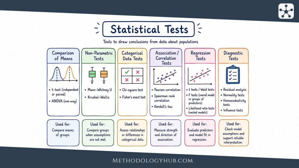
Common Tests Used in Hypothesis Testing
Different hypothesis tests are used for different research situations. The choice depends on the type of outcome variable, the number of groups or measurements, the design of the study, and the assumptions that can reasonably be made. A test that works well for comparing two independent means is not the same as a test for association between two categorical variables.
It helps to begin with the job each test performs. This chapter gives a compact overview of tests that appear often in introductory statistics, research methods courses, and academic articles. The following chapter then turns these tests into a selection process.
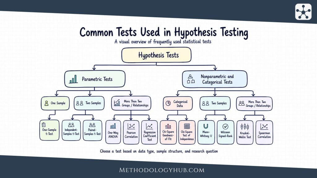
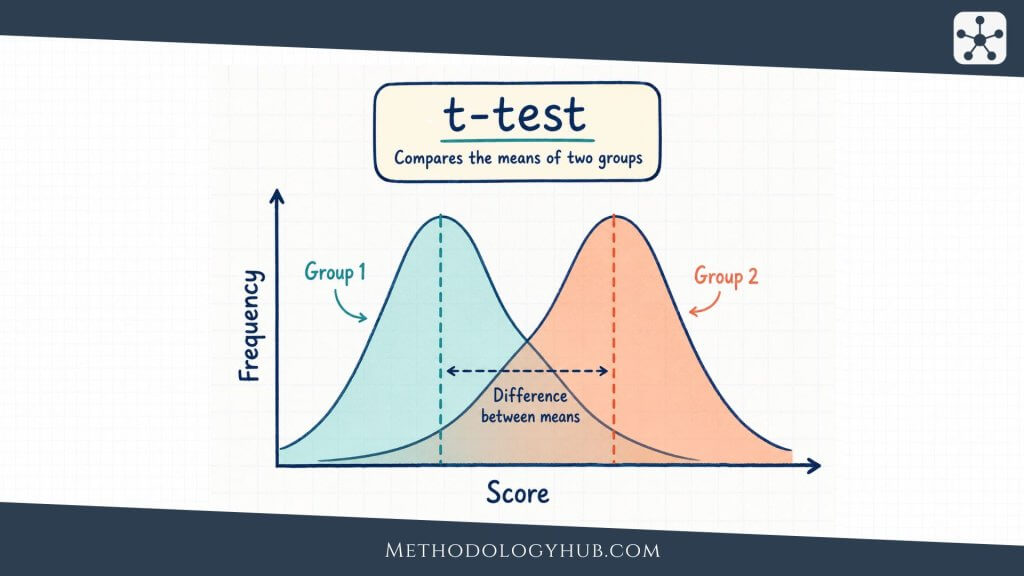
t-tests for means
A t-test is used when the research question focuses on a mean and the population standard deviation is unknown. A one-sample t-test compares a sample mean with a hypothesised population mean. For example, a researcher may test whether the average score of a sample differs from a known benchmark.
An independent-samples t-test compares the means of two independent groups. A teacher might compare exam scores between students taught with two different instructional approaches. A paired-samples t-test compares two related measurements, such as pre-test and post-test scores from the same students.
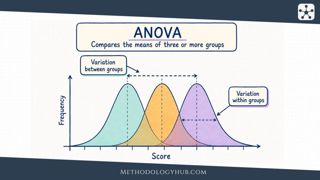
ANOVA for three or more group means
Analysis of variance, usually called ANOVA, is used when the researcher wants to compare means across three or more groups. A one-way ANOVA might compare average writing scores across three teaching methods. Instead of running several separate t-tests, ANOVA evaluates whether the group means differ more than would be expected from within-group variation.
When ANOVA is significant, researchers often follow it with post hoc comparisons to examine which groups differ from one another. Those follow-up comparisons should be chosen carefully because multiple testing can increase the chance of false positive findings.
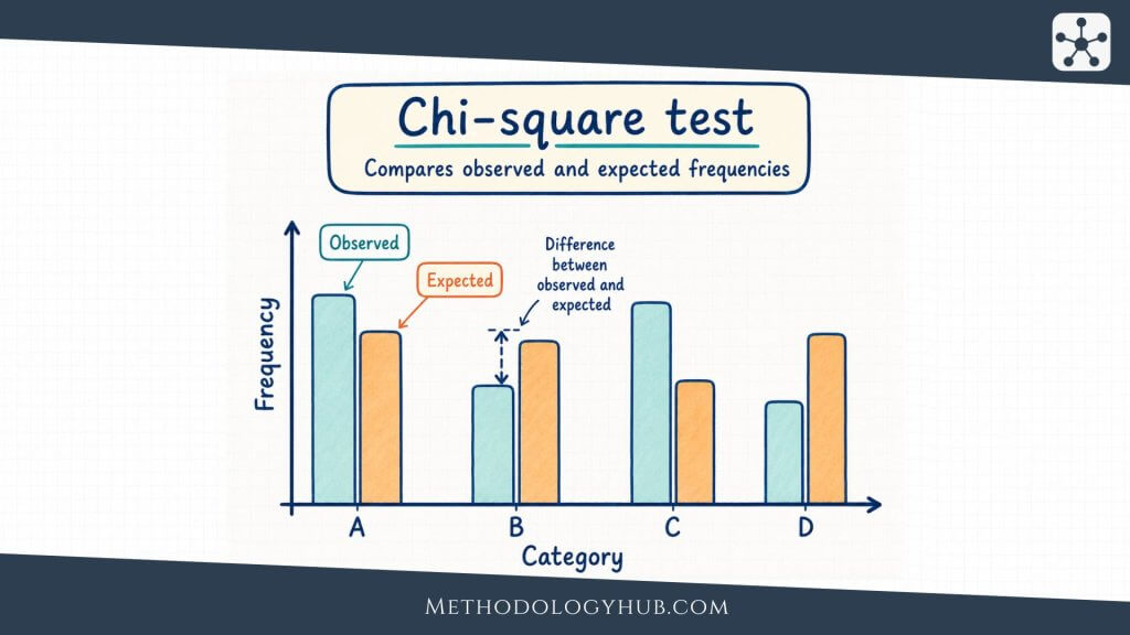
Chi-square tests for categorical data
Chi-square tests are used with categorical variables. A chi-square goodness-of-fit test compares observed counts with expected counts in one categorical variable. For example, a researcher might test whether students choose four essay topics equally often.
A chi-square test of independence examines whether two categorical variables are associated. For example, a researcher may test whether preferred study location is associated with year level in school. The test compares the observed counts in a table with the counts expected if the variables were independent.
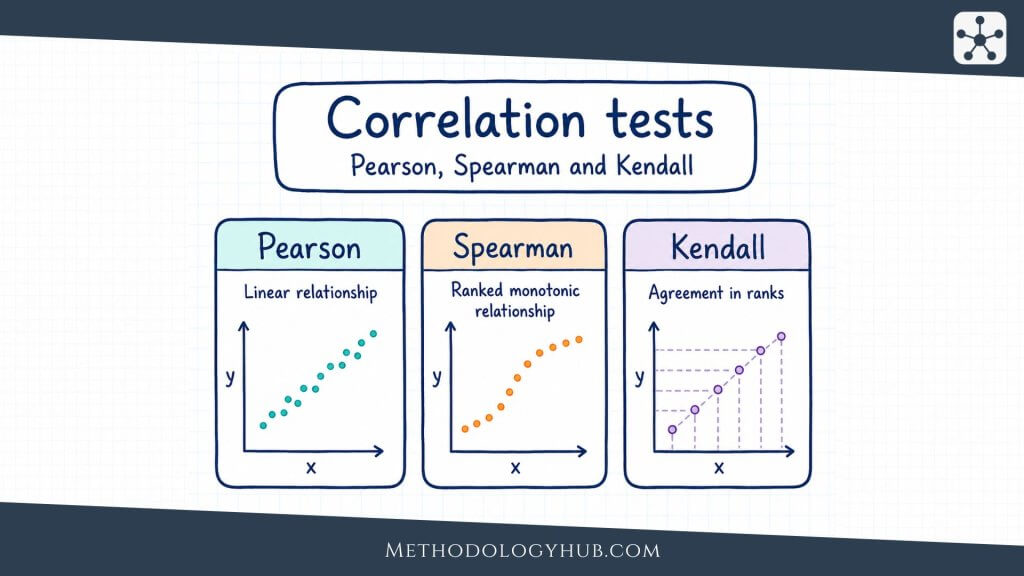
Correlation and regression tests
A correlation test examines whether two numerical variables are linearly associated. If a researcher studies the relationship between hours of study and exam scores, a correlation test can evaluate whether the observed correlation differs from zero in the population.
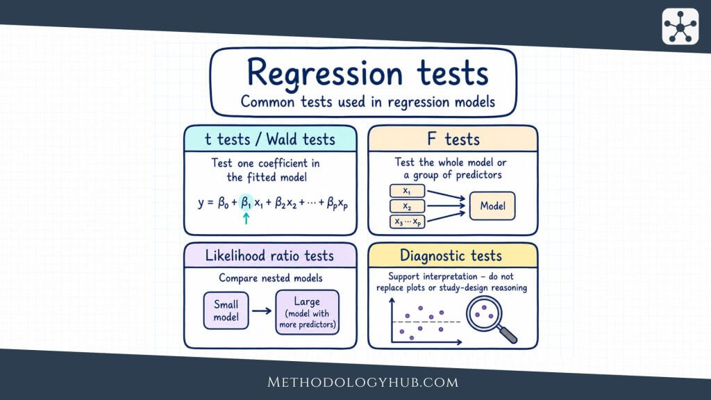
Regression tests extends this idea by modelling an outcome variable using one or more predictors. In simple linear regression, the hypothesis test for the slope asks whether the predictor is statistically associated with the outcome. In multiple regression, each coefficient is tested while holding the other predictors in the model constant.
Nonparametric tests
Nonparametric tests are often used when the assumptions of common parametric tests are not suitable for the data. For example, the Mann-Whitney U test can compare two independent groups when the outcome is ordinal or strongly non-normal. The Wilcoxon signed-rank test can be used for paired observations. The Kruskal-Wallis test can compare three or more independent groups.
These tests are not simply weaker substitutes. They answer slightly different questions and often work with ranks rather than raw values. The researcher should choose them because they fit the measurement level and distribution of the data, not only because another test did not produce the desired result.
| Research situation | Typical test | Main data type |
|---|---|---|
| One sample mean compared with a benchmark | One-sample t-test | Numerical outcome |
| Two independent group means | Independent-samples t-test | Numerical outcome, two groups |
| Two related measurements | Paired-samples t-test | Numerical outcome, paired data |
| Three or more group means | One-way ANOVA | Numerical outcome, categorical group variable |
| Association between two categorical variables | Chi-square test of independence | Categorical counts |
| Linear association between two numerical variables | Correlation test | Two numerical variables |
Choosing the Appropriate Hypothesis Test
Once the main tests are familiar, choosing among them becomes more manageable. The task is not to memorise a long list of test names. The task is to read the research question, identify the structure of the data, and match that structure to a method that answers the question directly.
This chapter follows the overview of common tests because selection is easier after the reader knows what each test is designed to do. The previous chapter answered, “What does each test do?” This chapter answers, “Given this question and this dataset, which test should be used?”
Start with the research question
The research question determines the kind of comparison or relationship being tested. A question about whether one average differs from a benchmark calls for a different test from a question about whether two categorical variables are associated. A question about a before-and-after change differs from a question about two unrelated groups.
Before choosing a test, the researcher should name the outcome variable, the explanatory variable if there is one, the comparison being made, and the unit of observation. This small step often solves much of the selection problem.
Identify the type of variable
Variable type is one of the strongest guides to test choice. Numerical outcomes, such as scores, times, heights, or scale totals, are often analysed with t-tests, ANOVA, correlation, or regression. Categorical outcomes, such as response categories or group memberships, often require chi-square tests or models designed for categorical data.
Measurement level should not be forced. If a variable contains categories, it should usually be treated as categorical. If a scale score has enough ordered values and behaves roughly like a numerical measure, numerical methods may be suitable. The decision should be explained clearly when the variable could be treated in more than one way.
Check the number of groups or measurements
The number of groups or measurements also directs test choice. One numerical sample compared with one known value suggests a one-sample t-test. Two independent groups suggest an independent-samples t-test. Two related measurements suggest a paired-samples t-test. Three or more independent groups suggest one-way ANOVA.
The word independent should be read carefully. Two groups are independent when the observations in one group are not naturally linked to observations in the other. Paired or related data occur when the same cases are measured twice, when participants are matched, or when observations come in natural pairs.
Examine the assumptions
Statistical tests depend on assumptions. For many parametric tests, the assumptions include independence of observations, an appropriate measurement scale, approximate normality in the relevant distribution or residuals, and sometimes similar variances across groups. For chi-square tests, expected cell counts should usually be large enough for the approximation to work well.
Assumptions should not be treated as a final checkbox after the result is known. They should influence the test choice. If assumptions are not reasonable, the researcher may need a different method, a transformation, a nonparametric test, a more suitable model, or a more cautious interpretation.
Use a test selection table
A test selection table is useful when it simplifies rather than replaces statistical reasoning. The table below gives a starting point for introductory research situations. It should be used with the research question, measurement level, study design, and assumptions in view.
| Question type | Data structure | Possible test |
|---|---|---|
| Is one mean different from a stated value? | One numerical sample | One-sample t-test |
| Do two independent groups differ in mean score? | Numerical outcome, two independent groups | Independent-samples t-test |
| Did scores change from before to after? | Two related numerical measurements | Paired-samples t-test |
| Do three or more groups differ in mean score? | Numerical outcome, three or more groups | One-way ANOVA |
| Are two categorical variables associated? | Counts in categories | Chi-square test of independence |
| Are two numerical variables linearly related? | Two numerical variables | Correlation test or regression |
7-Step Procedure for Hypothesis Testing
A standard procedure helps keep hypothesis testing clear and consistent. The steps do not turn statistics into a mechanical exercise, but they do prevent the researcher from jumping straight from a sample result to a conclusion. Each step has a separate job, and together they move from a research claim to a statistical decision.
The seven-step structure below is especially useful for students because it shows where the hypotheses, significance level, test choice, calculation, decision rule, and conclusion fit in the same process.

Step 1: State the null hypothesis, H0
The first step is to state the null hypothesis in statistical form. This usually means naming the population parameter and giving it a value or relationship. For a mean, the null hypothesis may look like H0: μ = 75. For a relationship, it may state that there is no association between two variables in the population.
The null hypothesis should be clear enough that the rest of the test can be built from it. A vague statement such as “there is no difference” is often not enough unless the variables, population, and parameter have already been defined.
Step 2: State the alternative hypothesis, Ha
The alternative hypothesis states what the test will support if evidence against H0 is strong enough. It can be two-sided, such as Ha: μ ≠ 75, or one-sided, such as Ha: μ > 75. The correct form depends on the research question.
This is also where the researcher decides whether the test is directional. If a study only has a reason to expect an increase, a greater-than alternative may be suitable. If both an increase and a decrease would be meaningful, a two-sided alternative is usually more appropriate.
Step 3: Set the significance level, α
The third step is to choose the significance level. In many introductory examples, α = 0.05. This threshold gives the decision rule for the test. If the p-value is less than or equal to α, the result is statistically significant under the chosen rule, and H0 is rejected.
The significance level should be chosen before looking at the final test result. Changing α after seeing the p-value weakens the logic of the procedure because the decision rule is no longer independent of the data.
Step 4: Collect data and choose the appropriate test
The fourth step connects the research design to the analysis. The researcher collects data using the planned method and then chooses a test that fits the research question, variable types, number of groups, dependence structure, and assumptions.
For example, if the outcome is a numerical score and the study compares two independent groups, an independent-samples t-test may be suitable. If the data are counts in categories, a chi-square test may be more appropriate. If the same participants are measured twice, the analysis should recognise the paired structure.
Step 5: Calculate the test statistic and p-value
The fifth step is the calculation stage. In hand calculations, this involves applying the test formula and finding the corresponding probability from a reference distribution. In most research settings, statistical software calculates the test statistic, degrees of freedom, and p-value.
The calculation should still be understood, even when software does the arithmetic. The researcher should know what the test statistic represents, what direction the effect has, and whether the p-value belongs to a one-tailed or two-tailed test.
Step 6: Construct acceptance and rejection regions or compare p-value to α
The sixth step applies the decision rule. In the critical-value approach, the researcher compares the test statistic with the critical value and checks whether it falls in the rejection region. In the p-value approach, the researcher compares the p-value directly with α.
Both approaches answer the same decision question. If the test statistic falls in the rejection region, or if p ≤ α, reject H0. If the test statistic does not fall in the rejection region, or if p > α, fail to reject H0.
Step 7: Draw a conclusion
The final step is to write the conclusion in terms of the research question. The conclusion should include the statistical decision and a plain-language interpretation. It should not say that the null hypothesis has been proven true. The correct wording is usually “reject H0” or “fail to reject H0.”
A strong conclusion also connects the result back to the design. For example, it may state that the sample provides evidence that the mean score differs from the benchmark, while noting that the conclusion applies to the population and conditions represented by the sample.
Interpretation of Results
Interpreting hypothesis testing results requires more than reading whether p is smaller than 0.05. The statistical decision is only one part of the interpretation. Researchers also need to consider the size of the effect, the confidence interval, the design of the study, and whether the assumptions of the test are reasonable.
This is where many results become clearer. A statistically significant result may be small in practical or academic terms. A non-significant result may still be uncertain if the sample was small. A p-value may help with the decision rule, but it does not carry the full meaning of the study.
Statistical significance
A result is statistically significant when the p-value is less than or equal to the chosen significance level. If α = 0.05 and p = 0.03, the researcher rejects H0. The result is considered statistically significant under that decision rule.
Statistical significance should be read as evidence against H0, not as proof that an effect is large, useful, or theoretically meaningful. A very large sample can make a small difference statistically significant. For that reason, the p-value should usually be reported with descriptive statistics and an effect size.
Non-significant results
A non-significant result occurs when the p-value is larger than α. If α = 0.05 and p = 0.18, the researcher fails to reject H0. This does not prove that there is no effect. It means the sample did not provide enough evidence to reject the null hypothesis using the chosen test and threshold.
Non-significant results can occur for several reasons. The null hypothesis may be close to the true situation. The effect may exist but be small. The sample may be too small. The measurements may be too variable. The chosen test may not fit the data well. For this reason, interpretation should be cautious and should not rely on a single phrase such as “no difference was found” without context.
Effect size
Effect size describes the magnitude of a result. In a comparison of two means, an effect size may show how large the difference is relative to variation in the data. In a correlation, the correlation coefficient itself gives information about direction and strength. In categorical analysis, measures such as risk difference, odds ratio, or Cramer’s V may be used.
Effect size helps readers understand the result as more than a yes-or-no decision. Two studies can have the same p-value but different effect sizes, or the same effect size but different p-values because of sample size. Reporting both gives a fuller interpretation.
Confidence intervals
Confidence intervals complement hypothesis testing by showing a range of plausible values for the population parameter. For example, a study might report a mean difference of 4 points with a 95% confidence interval from 1.2 to 6.8. This tells the reader not only that the difference is statistically significant if the interval excludes zero, but also the approximate size and precision of the estimate.
Wide intervals suggest more uncertainty. Narrow intervals suggest more precision. A confidence interval can also show when a non-significant result is still uncertain because the range includes both small and potentially meaningful values.
Reporting results in academic writing
Academic reporting should be precise enough that the reader can see the test, result, and interpretation. A short report often includes the test name, test statistic, degrees of freedom when relevant, p-value, effect size when available, and a sentence connecting the result to the research question.
For example, a t-test result may be reported as follows: “A one-sample t-test showed that the sample mean score differed from the benchmark, t(39) = 2.41, p = 0.021.” A fuller version might add the mean, standard deviation, confidence interval, and effect size. The exact format depends on the discipline and style guide.
Worked Example of Hypothesis Testing
A worked example can bring the full procedure together. Suppose a university department has a long-term average statistics quiz score of 70. A lecturer introduces a new set of practice exercises and wants to know whether students using the exercises have a different average score from the historical benchmark.
The lecturer collects scores from 40 students who used the practice exercises. The sample mean is 74.2, and the sample standard deviation is 10.5. Because the population standard deviation is unknown and the researcher is comparing one sample mean with a known benchmark, a one-sample t-test is suitable for this introductory example.
Step 1 and Step 2: State the hypotheses
The null hypothesis states that the population mean quiz score is equal to the benchmark of 70. The alternative hypothesis states that the population mean is different from 70. Because the lecturer is interested in any difference, not only an increase, the test is two-tailed.
- H0: μ = 70
- Ha: μ ≠ 70
Step 3 and Step 4: Set α and choose the test
The lecturer sets α = 0.05 before analysing the data. The outcome variable is numerical, the study has one sample, and the comparison is against a benchmark value. A one-sample t-test is therefore appropriate, assuming the scores are reasonably suitable for that test.
With n = 40, the degrees of freedom are n – 1 = 39. The test will compare the observed mean of 74.2 with the hypothesised mean of 70, while accounting for the sample standard deviation and sample size.
Step 5: Calculate the test statistic and p-value
The standard error is calculated as s / sqrt(n), which gives 10.5 / sqrt(40) = 1.66 approximately. The observed mean is 4.2 points above the benchmark. Dividing 4.2 by 1.66 gives a t statistic of about 2.53.
With 39 degrees of freedom, a two-tailed t-test with t = 2.53 gives a p-value of about 0.016. The exact value may vary slightly depending on rounding, but it remains below 0.05.
Step 6 and Step 7: Make the decision and write the conclusion
Because p = 0.016 is less than α = 0.05, the lecturer rejects H0. The sample provides statistically significant evidence that the population mean quiz score for students using the practice exercises differs from the historical benchmark of 70.
A careful academic interpretation might read: “A one-sample t-test indicated that the mean quiz score for students using the practice exercises was significantly different from the benchmark score of 70, t(39) = 2.53, p = 0.016. The sample mean was 74.2, suggesting a higher average score in this sample. This result should be interpreted in light of the study design, the sample, and the fact that the comparison uses a historical benchmark rather than random assignment to conditions.”
This final sentence keeps the conclusion proportionate. The test result supports rejecting the null hypothesis, but the design still affects what can be claimed. If the lecturer wanted stronger evidence about the practice exercises themselves, a study comparing students randomly assigned to exercise and non-exercise conditions would provide a stronger basis for causal interpretation.
Conclusion
Hypothesis testing gives researchers a structured way to evaluate claims with sample data. It begins with a null hypothesis and an alternative hypothesis, sets a significance level, uses an appropriate statistical test, and then compares the evidence with a decision rule. The procedure is useful because it keeps uncertainty visible rather than hiding it behind a single sample result.
The central ideas are connected. The null hypothesis provides the reference point. The test statistic measures how far the sample result is from that reference point. The p-value helps judge how unusual the result would be under the null hypothesis. Type I and Type II errors remind us that decisions can be wrong. Effect sizes and confidence intervals help turn the decision into a fuller interpretation.
The strongest use of hypothesis testing is careful rather than automatic. A statistically significant result should be read with its effect size, confidence interval, assumptions, and study design. A non-significant result should not be treated as proof that nothing exists. When these pieces are kept together, hypothesis testing becomes a disciplined way of reasoning from limited data.
FAQs on Hypothesis Testing
What is hypothesis testing?
Hypothesis testing is a statistical method used to evaluate a claim about a population by analysing sample data. It compares the observed result with what would be expected under a null hypothesis and then uses a decision rule based on a significance level or p-value.
What is the null hypothesis?
The null hypothesis, written as H0, is the starting statistical claim in a hypothesis test. It often states that there is no difference, no change, no association, or equality with a specified population value.
What is the alternative hypothesis?
The alternative hypothesis, written as Ha or H1, is the claim supported when the data provide enough evidence against the null hypothesis. It may state that a parameter is different from, greater than, or less than the value given in the null hypothesis.
What does the p-value mean in hypothesis testing?
The p-value is the probability of obtaining a result at least as extreme as the observed result, assuming the null hypothesis is true. A small p-value means the observed data would be relatively unusual under the null hypothesis.
What is the difference between Type I and Type II errors?
A Type I error occurs when a true null hypothesis is rejected. A Type II error occurs when a false null hypothesis is not rejected. The first is a false positive decision, while the second is a missed effect or missed difference.
How do you choose the right hypothesis test?
To choose the right hypothesis test, identify the research question, the type of outcome variable, the number of groups or measurements, whether the data are independent or paired, and the assumptions of the test. Numerical means, categorical counts, paired observations, and relationships between variables often require different tests.